Low- and high-dimensional logistic regression

Model specification

The logistic regression is a popular binary classifier and arguably the elementary building block of a neural network. Specifically, given a feature vector $\mathbf{x} \in \mathbb{R}^p$, the logistic regression models the binary outcome $y\in \{0,1\}$ as \begin{equation} \mathbb{P}(y=1 | \mathbf{x} ; b, \boldsymbol \theta) = \frac{1}{1+ \exp\big( -(b + \boldsymbol\theta’\mathbf{x}) \big)} = : \Lambda ( b + \boldsymbol \theta’\mathbf{x}), \label{eq:LogisticModel} \tag{1} \end{equation} where we introduced the sigmoid function $\Lambda(x) = \frac{1}{1+\exp(-x)}$ in the last equality. The step-wise explanation of the logistic regression is: (1) introduce the parameter vector $\boldsymbol{\theta}\in\mathbb{R}^p$ to linearly combine the input features into the scalar $\boldsymbol \theta’\mathbf{x}$, (2) add the intercept/bias parameter $b$, and (3) transform $b+\boldsymbol \theta’\mathbf{x}$ into a probability by guiding it through the sigmoid function.¹ Figure 1 clearly shows how the sigmoid function maps any input into the interval (0,1) thereby resulting in a valid probability.

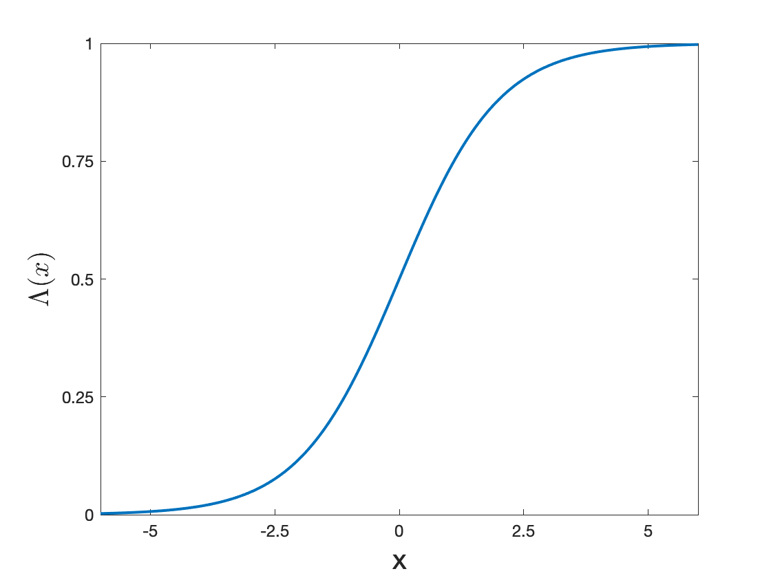
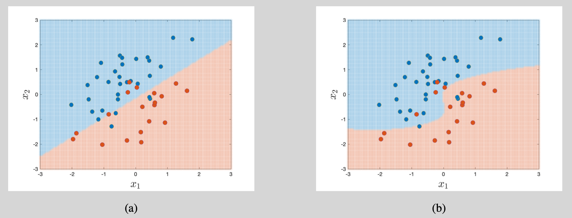
To provide a geometrical interpretation of the logistic regression, we note that $\Lambda(x)\geq0.5$ whenever $x\geq 0$. If we label an outcome as 1 whenever its probability $\mathbb{P}(y=1 | \mathbf{x} ; b, \boldsymbol \theta)$ exceeds 0.5 (majority voting), then the label 1 is assigned whenever $b + \boldsymbol\theta’\mathbf{x}\geq 0$. Two illustrations are provided in Figure 2.

General remarks on maximum likelihood estimation

The following two identities will be especially convenient when developing the maximum likelihood framework: (1) $1-\Lambda(x)=\frac{1}{1+\exp(x)}=\Lambda(-x)$, and (2) $\frac{d}{dx} \Lambda(x) =\big(1+\exp(-x)\big)^{-2}\times \exp(-x)= \Lambda(x)\big( 1 -\Lambda(x) \big)$. Exploiting the first identity, the likelihood function for $n$ independent observations $\big(y_i, \mathbf{x}_i \big)_{i=1,\ldots,n}$ from model \eqref{eq:LogisticModel} can be written as $$ \begin{aligned} L(b,\boldsymbol\theta) &= \prod_{i=1}^n \Big(\Lambda ( b + \boldsymbol \theta’\mathbf{x}_i)\Big)^{y_i} \Big(1-\Lambda ( b + \boldsymbol\theta’\mathbf{x}_i)\Big)^{1-y_i} \\ &= \prod_{i=1}^n \Lambda\Big( (2y_i -1) \big( b + \boldsymbol\theta’\mathbf{x}_i \big) \Big). \end{aligned} $$ Clearly, the implied log-likelihood function is $$ \log L(b,\boldsymbol \theta) = \sum_{i=1}^n \log \Lambda \Big( (2y_i -1) \big( b + \boldsymbol \theta’\mathbf{x}_i \big) \Big). $$ The second identity is subsequently used to easily compute the derivatives of this scaled log-likelihood. Repeated application of the chain rule gives the gradients $$ \begin{aligned} \frac{\partial \log L(b,\boldsymbol\theta) }{\partial b} &= \sum_{i=1}^n \frac{1}{\Lambda\Big( (2y_i -1) \big( b + \boldsymbol\theta’\mathbf{x}_i \big) \Big)} \Lambda\Big( (2y_i -1) \big( b + \boldsymbol\theta’\mathbf{x}_i \big) \Big)\Big[1 - \Lambda\Big( (2y_i -1) \big( b + \boldsymbol\theta’\mathbf{x}_i \big)\Big) \Big] (2y_i -1) \\ &= \sum_{i=1}^n (2y_i -1) \Big[1 - \Lambda\Big( (2y_i -1) \big( b + \boldsymbol\theta’\mathbf{x}_i \big) \Big) \Big], \\ \frac{\partial \log L(b,\boldsymbol \theta) }{\partial \boldsymbol\theta} &= \sum_{i=1}^n (2y_i -1) \mathbf{x}_i \Big[1 - \Lambda\Big( (2y_i -1) \big( b + \boldsymbol\theta’\mathbf{x}_i \big) \Big) \Big]. \end{aligned} $$ The stack of these two gradients will be denoted as $\mathbf{S}(b,\boldsymbol\theta)= \sum_{i=1}^n (2y_i -1) \left[\begin{smallmatrix} 1 \\ \mathbf{x}_i \end{smallmatrix}\right] \Big[1 - \Lambda\Big( (2y_i -1) \big( b + \boldsymbol\theta’\mathbf{x}_i \big) \Big) \Big]$. As these gradients are linear in $\Lambda\big( (2y_i -1) \big( b + \boldsymbol\theta’\mathbf{x}_i \big) \big)$, the $(p+1)\times(p+1)$ Hessian matrix follows as

\begin{equation} \begin{aligned} \mathbf{H}(b, \boldsymbol\theta) &= \left[\begin{smallmatrix} \frac{\partial^2 \log L(b,\boldsymbol\theta) }{\partial b^2} & \frac{\partial^2 \log L(b,\boldsymbol\theta) }{\partial b \partial \boldsymbol\theta’} \\ \frac{\partial^2 \log L(b,\boldsymbol\theta) }{\partial b \partial \boldsymbol\theta} & \frac{\partial^2 \log L(b,\boldsymbol \theta) }{\partial \boldsymbol \theta \partial \boldsymbol \theta’} \end{smallmatrix}\right] \\ &= -\sum_{i=1}^n \left[\begin{smallmatrix} 1 & \mathbf{x}_i’ \\ \mathbf{x}_i & \mathbf{x}_i \mathbf{x}_i’\end{smallmatrix}\right] \Lambda\Big( (2y_i -1) \big( b + \boldsymbol \theta’\mathbf{x}_i \big)\Big) \Big[1 - \Lambda\Big( (2y_i -1) \big( b + \boldsymbol\theta’\mathbf{x}_i \big) \Big) \Big], \end{aligned} \end{equation} where $(2 y_i-1)^2=1$ has been used. Finally, take an arbitrary $\mathbf{a} = (a_0,a_1,\ldots, a_p)’\in \mathbb{R}^{p+1}$, then \begin{equation} \mathbf{a}’ \mathbf{H}(b, \boldsymbol\theta)\mathbf{a} = - \sum_{i=1}^n (a_0 + \mathbf{a}_{1:p}’\mathbf{x}_i)^2 \Lambda\Big( (2y_i -1) \big( b + \boldsymbol\theta’\mathbf{x}_i \big)\Big) \Big[1 - \Lambda\Big( (2y_i -1) \big( b + \boldsymbol\theta’\mathbf{x}_i \big) \Big) \Big], \label{eq:PosDefHession} \tag{2} \end{equation} with $\mathbf{a}_{1:p}= (a_1,\ldots,a_p)^\prime$. We make several observations related to \eqref{eq:PosDefHession}:

1. The sigmoid function satisfies $0 < \Lambda(x) < 1$ for all $x$. Each term within the summation is thus non-negative.
2. The equality $\mathbf{a}’ \mathbf{H}(b, \boldsymbol\theta) \mathbf{a} =0$ holds if and only if $a_0 + \mathbf{a}_{1:p}’\mathbf{x}_i=0$ for all $i\in{1,2,\ldots,n}$. Or equivalently, $\mathbf{a}’ \mathbf{H}(b, \boldsymbol\theta) \mathbf{a} =0$ if and only if $\mathbf{a}$ is orthogonal to all vectors in the collection \begin{equation} \left\{\begin{bmatrix} 1 \\ \mathbf{x}_1 \end{bmatrix}, \begin{bmatrix} 1 \\ \mathbf{x}_2 \end{bmatrix}, \ldots, \begin{bmatrix} 1 \\ \mathbf{x}_n \end{bmatrix} \right\}. \label{eq:vectorset} \tag{3} \end{equation} This analysis naturally leads to two important regimes.

Low-dimensional: If $p$ is small, then $\mathbf{a}’ \mathbf{H}(b, \boldsymbol\theta) \mathbf{a}$ is strictly negative. The objective function is strictly concave because the Hessian matrix is negative-definite. The likelihood function has an unique minimizer and asymptotically valid inference is possible.

High-dimensional: If $p$ is large, then we enter a high-dimensional regime with (1) many parameters to estimate, and (2) a Hessian matrix with eigenvalues (close to) 0. The dimensionality of the problem requires faster algorithms and parameter regularization.

The low-dimensional regime

Estimation

Let us denote the maximum likelihood estimators by $\hat b$ and $\hat{\boldsymbol\theta}$. These estimators are the solutions of $$ \mathbf{S}(\hat b, \hat{\boldsymbol\theta})= \sum_{i=1}^n (2y_i -1)\begin{bmatrix} 1 \\ \mathbf{x}_i \end{bmatrix} \Big[1 - \Lambda\Big( (2y_i -1) \big( \hat b + \hat{\boldsymbol \theta}’\mathbf{x}_i \big) \Big) \Big] = \mathbf{0}. $$ The solution to this set of equations is not available in closed form and we thus need to resort to numerical methods. The maximization of strictly concave objective functions is well-studied and numerical solution schemes are readily available. Especially for small $p$ (say $p<50$ and $p«n$), we can rely on the Newton-Rhapson algorithm. The sketch of the algorithm is as follows:

1. Make a starting guess for the parameters, say $b_{\{0\}}$ and $\boldsymbol\theta_{\{0\}}$.

2. Iteratively update the parameters based on a quadratic approximation of log-likelihood. That is, being located at the point $\big\{b_{\{i\}},\boldsymbol\theta_{\{i\}}\big\}$, the local quadratic approximation of the log-likelihood (read: its second order Taylor expansion) is \begin{equation} L(b,\boldsymbol \theta) \approx \log L(b_{\{i\}},\boldsymbol \theta_{\{i\}}) + \mathbf{S}(b_{\{i\}},\boldsymbol\theta_{\{i\}})^\prime \begin{bmatrix} b - b_{\{i\}} \\ \boldsymbol{\theta}-\boldsymbol{\theta}_{\{i\}} \end{bmatrix} + \frac{1}{2} \begin{bmatrix} b - b_{\{i\}}\\ \boldsymbol\theta - \boldsymbol\theta_{\{i\}} \end{bmatrix}^\prime \mathbf{H}(b_{\{i\}}, \boldsymbol\theta_{\{i\}})\begin{bmatrix} b - b_{\{i\}}\\ \boldsymbol\theta - \boldsymbol\theta_{\{i\}} \end{bmatrix}. \end{equation}

   The updates $b_{\{i+1\}}$ and $\boldsymbol{\theta}_{\{i+1\}}$ are the optimizers of this quadratic approximation, or \begin{equation} \begin{bmatrix} b_{\{i+1\}}\\ \boldsymbol \theta_{\{i+1\}} \end{bmatrix} = \begin{bmatrix} b_{\{i\}}\\ \boldsymbol \theta_{\{i\}} \end{bmatrix} - \big[ \mathbf{H}(b_{[i]},\boldsymbol\theta_{\{i\}}) \big]^{-1} \mathbf{S}(b_{\{i\}},\boldsymbol\theta_{\{i\}}). \label{eq:NewtonRhapsonUpdate} \tag{4} \end{equation}

3. Repeatly update the parameter values using \eqref{eq:NewtonRhapsonUpdate} until (relative) parameter changes become negligible.

In typical settings the Newton-Rhapson algorithm converges after a small number of iterations.

Asymptotically valid inference

Define $\hat{\boldsymbol \gamma} = \left[\begin{smallmatrix} \hat{b} \\ \hat{\boldsymbol\theta} \end{smallmatrix}\right]$ and $\boldsymbol \gamma = \left[\begin{smallmatrix} b \\ \boldsymbol\theta \end{smallmatrix}\right]$. Results as in McFadden and W.K. Newey (1994) imply: $$ \sqrt{n}\left( \hat{\boldsymbol \gamma} - \boldsymbol \gamma \right) \stackrel{D}{\to} \mathcal{N}(\mathbf{0}, \mathbf{J}^{-1}) \quad \text{as} \quad T\to\infty, \label{eq:AsymptoticDistr} \tag{5} $$ where $\mathbf{J}= - \mathbb{E}\left[ \frac{\partial^2 \log \Lambda\big( (2y-1) (b+\boldsymbol\theta’\mathbf{x}) \big) }{\partial \boldsymbol \gamma \partial \boldsymbol \gamma’} \right]$ (the expectation is computed w.r.t. the joint distribution of $(y,\mathbf{x})$). A consistent estimator for $\mathbf{J}$, for example $$ \hat{\mathbf{J}} = \frac{1}{n}\mathbf{H}(\hat b, \hat{\boldsymbol\theta}) =-\frac{1}{n}\sum_{i=1}^n \left[\begin{smallmatrix} 1 & \mathbf{x}_i’ \\ \mathbf{x}_i & \mathbf{x}_i \mathbf{x}_i’\end{smallmatrix}\right] \Lambda\Big( (2y_i -1) \big( \hat{b} + \hat{\boldsymbol \theta}’\mathbf{x}_i \big)\Big) \Big[1 - \Lambda\Big( (2y_i -1) \big( \hat b + \hat{\boldsymbol\theta}’\mathbf{x}_i \big) \Big) \Big], $$ is an almost immediate byproduct of the Newton-Rhapson algorithm. Asymptotically valid hypothesis tests are thus easy to construct in this low-dimensional regime.

Illustration 1: Haberman’s survival data set

The data is freely available here, or you can readily download the SQL-file $\texttt{HabermanDataSet.sqlite}$ from my GitHub page. The binary variable in this study is the survival status of $n=306$ patients who had undergone surgery for breast cancer. For $i=1,\ldots,n$, we recode this variable into $y_i=1$ (patient $i$ survived 5 years or longer) and $y_i=0$ (patient $i$ died within 5 years). There are three explanatory variables:

1. $Age_i$: age of patient $i$ at the time of operation
2. $Year_i$: year of operation for patient $i$ with offset of 1900 (i.e. the year 1960 is recorded as 60)
3. $AxilNodes_i$: number of axillary nodes detected in patient $i$

Following Landwehr et al. (1984), we look at the following model specification $$ \mathbb{P}(y_i=1 | \mathbf{x}_i ; b, \boldsymbol\theta) = \Lambda\Big( b + \theta_1 z_{1i} + \theta_2 z_{1i}^2 + \theta_3 z_{1i}^3 + \theta_4 z_{2i} + \theta_5 z_{1i} z_{2i} + \theta_6 \log(1+AxilNodes_i) \Big), $$ where $z_{1i}=Age_{i}-52$ and $z_{2i} = Year_{i} - 63$.² The estimation results are listed in Tables 2–3 and Figure 3. Some short comments are:

• The levels of $z_1$ and $z_2$ do not significantly influence the 5-year survival probability. These features can be omitted from the model.
• The sigmoid function is monotonically increasing. An increase in $b + \theta_1 z_{1i} + \theta_2 z_{1i}^2 + \theta_3 z_{1i}^3 + \theta_4 z_{2i} + \theta_5 z_{1i} z_{2i} + \theta_6 \log(1+AxilNodes_i)$ will thus imply a higher survival probabiliy. The estimation results point towards nonlinear effect in $Age$. Generally speaking, older people are at a higher risk but this effect is not strictly monotone (Figure 3).³
• The accuracy, the fraction of correctly classified cases, is $235/305\approx 77.1\%$. Further classification details are shown in Table 3.

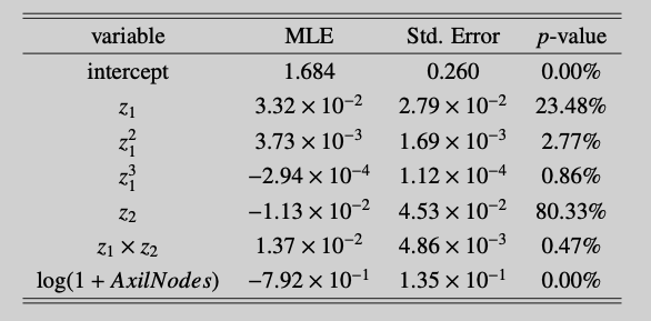
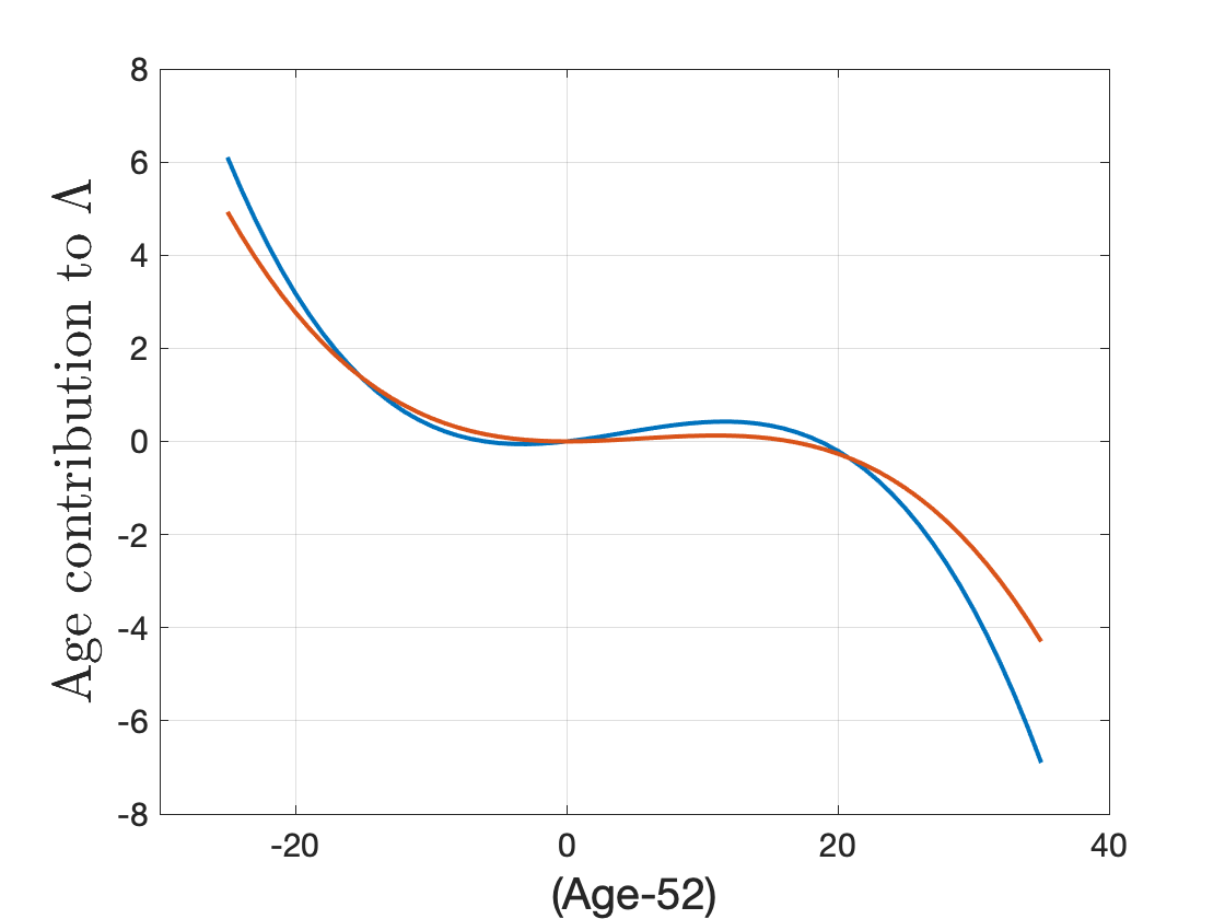
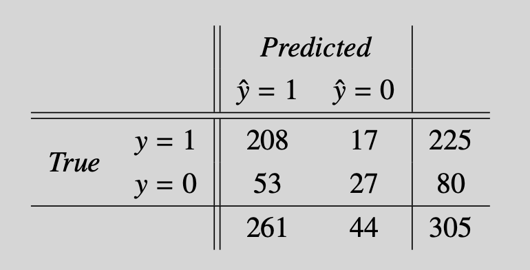
Illustration 2: A Monte Carlo study to compare implementations

We also study the low-dimensional logistic regression through two small Monte-Carlo studies. The settings are outlined below.

DGP 1: Comparing languages

The data features two regressors, $\mathbf{x}_i = (x_{1i},x_{2i})^\prime$, generated as $\mathbf{x}_i\stackrel{i.i.d.}{\sim} \mathcal{N}(\mathbf{0}, \boldsymbol{\Sigma})$ with $\boldsymbol{\Sigma}= \left[ \begin{smallmatrix} 1 & \rho \\ \rho &1 \end{smallmatrix} \right]$. The binary outcome $y_i\in\{0,1\}$ takes the value 1 with probability $\Lambda(b + \boldsymbol\theta’ \mathbf{x}_i)$. The selected parameters are: $\rho=0.3$, $b=0.5$, $\theta_1=0.3$ and $\theta_2=0.7$. For $n\in\{200,500\}$, we compare the following methods:

• Direct Newton-Rhapson implementations in Matlab, Numpy, R and TensorFlow. The implementations and convergence criteria are exactly the same across programming languages.
• The logistic regression implementations from GLM (R) and Scikit-learn (Python).

For each setting, the code will (1) generate the data, (2) optimize the log-likelihood to compute the MLE, and (3) construct the asymptotically valid t-statistic based on the limiting distribution in \eqref{eq:AsymptoticDistr}.⁴ We repeat the procedure $N_{sim}=1000$ times.

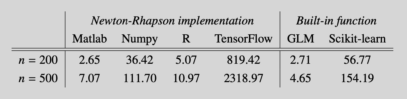
Computational times are reported in Table 4. Using $a>b$ to denote $a$ being faster than $b$, we have $Matlab>R>Python>TensorFlow$. The ranking of the first three has been the same in my other posts as well. As the Newton-Rhapson algorithm relies mainly on linear algebra, the good performance of Matlab (originally a linear algebra platform) might not come as a surprise. The poor performance of TensorFlow is perhaps rather unexpected. Possible explanations are: the manual implementation through $\texttt{tf.linalg}$ not allowing pieces of the code to be executed in faster lower level languages, and inefficiencies in the TensorFlow linear algebra implementation. The latter has been reported by Sankaran et al. (2022).

The built-in function have similar performances to their manually implemented counterparts. Their implementation is probably faster but the built-in function incur some overhead costs.

DGP 2: Adding irrelevant features to increase $p$

Consider $\mathbf{x}_i = (x_{1i},\ldots,x_{pi})^\prime\stackrel{i.i.d.}{\sim} \mathcal{N}(\mathbf{0}, \boldsymbol \Sigma)$. The $(p\times p)$ matrix $\boldsymbol \Sigma$ takes value 1 on the main diagonal and $\rho$ on each off-diagonal element. The additional parameters are $b=0.5$, $\theta_1=0.3$, $\theta_2=0.7$ and $\theta_3=\ldots=\theta_p=0$. Again, the binary outcome $y_i\in\{0,1\}$ takes the value 1 with probability $\Lambda(b + \boldsymbol\theta’ \mathbf{x}_i)$. We fix $n=200$ but vary $\rho\in\{0.3,0.8 \}$ and $p\in\{2,3,\ldots,20\}$.

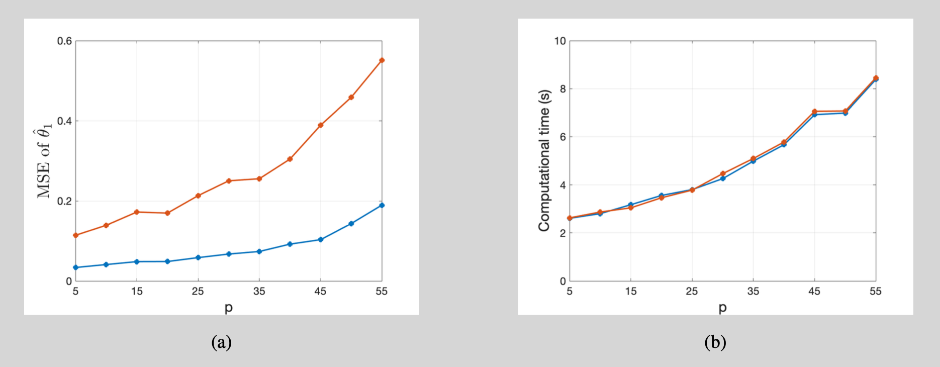
Some comments on Figure 4 are:

• More features make it more difficult to determine which explanatory variables are driving the success probability. The mean squared error of the parameter estimators increases. This effect amplifies if the regressors are more correlated (increasing $\rho$).
• Computational times increase faster than linear in $p$. The correlation parameter $\rho$ does not influence computational times.

The high-dimensional regime

Two issues arise when $p$ becomes larger:

Issue 1: If $p>n$, then there exist vectors that are orthogonal to all vectors in \eqref{eq:vectorset}. The likelihood is flat in these directions and the maximum likelihood estimator is no longer uniquely defined. In practice, performance typically deteriorates earlier. As soon as $p$ and $n$ are of similar orders of magnitude, then decreased curvature in the objective function causes additional noise to start leaking into the estimator. These effects are more pronounced when the regressors are more correlated.

Issue 2: The computational costs of the objective function do not scale well with increasing $p$. That is, calculating $\big[ \mathbf{H}(b_{[i]},\boldsymbol\theta_{\{i\}}) \big]^{-1}$ becomes increasingly time-consuming because standard matrix inversion algorithms have a computational complexity of about $\mathcal{O}(p^3)$.

Regularization is the typical solution to the first issue. In this post we will consider $L_1$- and $L_2$-regularization. The algorithmic modifications originate from findings in Tseng (2001). The results in this paper guarantee the convergence of a cyclic coordinate descent method whenever the objective function is a sum of a convex function and a seperable function.⁵ These repeated updates of single coordinates/parameters will decrease computational costs by avoiding issue 2.

Regularization with $L_2$-penalty

We start with $L_2$-regularization because it is easiest to explain. The objective function adds an additional penalty term $\lambda \|\boldsymbol \theta\|_2^2=\lambda \sum_{j=1}^p \theta_j^2$ to the previous negative log-likelihood. The estimators for $b$ and $\boldsymbol \theta$ are now the minimizers of \begin{equation} Q_\lambda(b,\boldsymbol \theta) = \sum_{i=1}^n \log \Lambda \Big( (2y_i -1) \big( b + \boldsymbol \theta’\mathbf{x}_i \big) \Big) + \lambda \|\boldsymbol \theta\|_2^2. \label{eq:L2ObjectiveFunction} \tag{6} \end{equation} The intercept parameter $b$ is not penalized.⁶ There are (at least) two intuitive explanations for the penalty term $\lambda \|\boldsymbol \theta\|_2^2$:

1. The Hessian of the penalty term with respect to the parameter vector $\boldsymbol \theta$ is $\frac{\partial^2}{\partial \boldsymbol \theta \partial \boldsymbol \theta^\prime} \lambda \|\boldsymbol \theta\|_2^2 = 2 \lambda \boldsymbol{I}_p$. The penalty term adds additional curvature to the objective function and thus provides a better defined minimum.
2. The $L_2$-penalty discourages parameter solutions with a large norm. This avoids overfitting. For example, with strongly positively correlated variables it occurs that excessively positive and excessively negative parameters mostly cancel out to only describe small and noisy effects. These large parameter vectors marginally improve the fit but cause high variance. This situation is avoided if parameter vectors with a high norm are penalized.

Given the validity of cyclic coordinate descent, the solution algorithm for optimization problem is relatively straightforward:

1. Make a starting guess for the parameters, say $b_{\{0\}}$ and $\boldsymbol\theta_{\{0\}}$.
2. We cycle through each $k\in\{1,2,\ldots,p\}$ and determine the parameter value $\theta_k$ with the lowest value for $Q_\lambda(b,\boldsymbol \theta)$. To clarify, we split the vector $\boldsymbol \theta$ into its $k$^th component $\theta_k$, and a vector with its $k$^th component being omitted, i.e. $\boldsymbol \theta_{-k}=(\theta_1,\ldots,\theta_{k-1},\theta_{k+1},\ldots,\theta_p)^\prime$ (and similar notational conventions for $\boldsymbol x_i$). The new single-parameter objective function reads \begin{equation} Q_\lambda^*(\theta_k) = \sum_{i=1}^n \log \Lambda \Big( (2y_i -1) \big( b + \boldsymbol \theta_{-k}’\mathbf{x}_{i,-k}+\theta_k x_{i,k} \big)\Big)+\lambda \theta_k^2 +\lambda\|\boldsymbol\theta_{-k} \|_2^2, \end{equation} where the last contribution $\lambda\|\boldsymbol\theta_{-k} \|_2^2$ is irrevelvant to the solution. This univariate problem is easily solved using the Newton-Rhapson algorithm. We stress that any parameter update continues to be used in the subsequent coordinate descents.
3. Update the intercept parameter $b$ using Newton-Rhapson.
4. Repeat steps 2 and 3 until the (relative) changes in all parameters are negligible.

References

J.M. Landwehr, D. Pregibon and A.C. Shoemaker (1984), Graphical Methods for Assessing Logistic Regression Models, Journal of the American Statistical Association

D. McFadden and W.K. Newey (1994), Large Sample Estimation and Hypothesis Testing, Chapter 36, Handbook of Econometrics

A. Sankaran, N.A. Alashti and C. Psarras (2022), Benchmarking the Linear Algebra Awareness of TensorFlow and PyTorch, arXiv:2202.09888

P. Tseng (2001), Convergence of a Block Coordinate Descent Method for Nondifferentiable Minimization, Journal of Optimization Theory and Applications

Notes