The Vasiček short-rate model

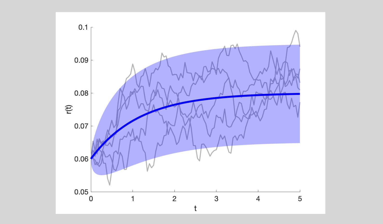
The Vasiček model is an interest rate model which specifies the short rate $r(t)$ under the risk-neutral dynamics (or $\mathbb{Q}$-dynamics) as \begin{equation} dr(t) = \kappa \big( \theta -r(t)\big) dt + \sigma dW(t), \tag{1} \label{eq:Vasicek_dif_eq} \end{equation} with initial condition $r(0) = r_0$ and $W(t)$ denoting a standard Brownian motion driving the stochastic differential equation. An explicit expression for $r(t)$ can be derived using Itô calculus (see, e.g. Mikosch (1998); Chapter 3). To solve \eqref{eq:Vasicek_dif_eq}, we try the solution $f\big(r(t),t\big) = r(t) e^{\kappa t}$. The Itô lemma implies \begin{equation} \begin{aligned} df\big(r(t),t\big) &= \kappa r(t) e^{\kappa t} dt + e^{\kappa t} dr(t) \\ &= \kappa r(t) e^{\kappa t} dt + e^{\kappa t}\Big[ \kappa \big( \theta -r(t)\big) dt + \sigma dW(t)\Big] \\ &= \kappa \theta e^{\kappa t} dt + \sigma e^{\kappa t} dW(t). \end{aligned} \tag{2} \label{eq:ItoLemmaSolved} \end{equation} The RHS of \eqref{eq:ItoLemmaSolved} no longer depends on $r(t)$ and we can thus integrate to find expressions for $f\big(r(t),t\big)$. This result is important for two reasons. First, we can integrate over the range $[0,t]$ to find $$ \begin{aligned} f\big( r(t), t \big) &- f\big( r(0),0\big) = r(t) e^{\kappa t} -r_0 = \int_0^t df\big( r(s),s\big) \\ &= \int_0^t \kappa \theta e^{\kappa s} ds + \int_0^t \sigma e^{\kappa s} dW(s). \end{aligned} $$ After some rearrangments the explicit solution for $r(t)$ is \begin{equation} r(t) = r_0 e^{-\kappa t} + e^{-\kappa t} \int_0^t \kappa \theta e^{\kappa s} ds + e^{-\kappa t} \int_0^t \sigma e^{\kappa s} dW(s). \label{eq:rtexplicit} \tag{3} \end{equation} With this explicit expression for $r(t)$ we can calculate its mean and variance. Since stochastic integrals have zero mean we have $$ \begin{aligned} \mathbb{E}\big[ r(t) \big] &= r_0 e^{-\kappa t} + \theta e^{-\kappa t} \left[ e^{\kappa t} -1 \right] = r_0 e^{-\kappa t} + \theta \left[ 1-e^{-\kappa t} \right] \\ &=: r_0 e^{-\kappa t} + \theta \kappa \Lambda(t), \end{aligned} $$ where we defined $\Lambda(t) = \int_0^t e^{-\kappa s} ds = \frac{1}{\kappa}\left[ 1 - e^{-\kappa t} \right]$. The long-run mean of the process is $\lim_{t\to\infty} \mathbb{E}\big[ r(t) \big] = \theta$. Moreover, by Itô isometry the variance of the process is $$ \mathbb{V}\text{ar}\big[r(t)\big] = \sigma^2 e^{-2\kappa t} \int_0^t e^{2\kappa s} ds = \tfrac{\sigma^2}{2\kappa} \left[ 1- e^{-2\kappa t} \right] = \tfrac{1}{2} \sigma^2 \Lambda(2t). $$ Second, \eqref{eq:ItoLemmaSolved} is the starting point to derive an exact discretization of $r(t)$. Such a discretization will allow us to simulate paths of $r(t)$ that can later be used to value interest rate derivatives. Given a time step $h$, we now integrate \eqref{eq:ItoLemmaSolved} over the interval $[t-h,t]$ to obtain $$ \begin{aligned} f &\big( r(t), t \big) - f\big( r(t-h),t-h\big) = \int_{t-h}^t df\big( r(s),s\big) \\ &= \theta \big( e^{\kappa t} - e^{\kappa(t-h)}\big) + \int_{t-h}^t \sigma e^{\kappa s} dW(s) \\ & \iff r(t) = \theta \big(1-e^{-\kappa h}\big) +e^{-\kappa h}r(t-h) + e^{-\kappa t} \int_{t-h}^t \sigma e^{\kappa s} dW(s). \end{aligned} $$ The discretized process of $r(t)$ thus follows an AR(1) model with intercept $\theta \big(1-e^{-\kappa h}\big)$, autoregressive coefficient $e^{-\kappa h}$, and innovation process $e^{-\kappa t} \int_{t-h}^t \sigma e^{\kappa s} dW(s)$. These innovations have some interesting properties. First, note how the integration intervals of subsequent steps of the discretization do not overlap. For example, $\int_{t-h}^t \sigma e^{\kappa s} dW(s)$ depends on $ \{ W(s) : t-h \leq s \leq t \}$, whereas $\int_{t}^{t+h} \sigma e^{\kappa s} dW(s)$ depends on $\{W(s) : t \leq s \leq t+h \}$. With increments of Brownian motions being independent, we must conclude that these stochastic integrals are independent. Second, stochastic integrals are normally distributed and mean zero. The distributions of the innovations is thus fully specified after computing its variance, or $$ \begin{aligned} \mathbb{V} &\text{ar}\left[ e^{-\kappa t} \int_{t-h}^t \sigma e^{\kappa s} dW(s) \right] \\ &= \sigma^2 e^{-2\kappa t} \int_{t-h}^t e^{2\kappa s} ds = \tfrac{\sigma^2}{2\kappa }\left[ 1 - e^{-2\kappa h} \right] = \sigma^2 h \left[ \frac{e^{-2\kappa h}-1}{-2\kappa h} \right] \\ &=: \sigma^2 h \alpha\big( -2\kappa h \big), \end{aligned} $$ where we defined $\alpha(x)=\tfrac{e^x-1}{x} \text{ with }\alpha(0)=0$. Overall, we can simulate data from the Vasiček model using $r(0)=r_0$ as the starting value and moving forward according to the recursion \begin{equation} r(t) = \theta \kappa \Lambda(h) + e^{-\kappa h} r(t-h) + u_t^{(h)},\; u_t^{(h)}\stackrel{i.i.d.}{\sim}\mathcal{N}\left(0, \sigma^2 h \alpha\big( -2\kappa h \big)\right). \label{eq:vasiceksteps} \end{equation} Some sample paths of the Vasiček model are displayed in Figure 1.

Risk-neutral valuation of a zero-coupon bond

Let $X$ denote a contingent claim with maturity date $T$. According to the risk-neutral valuation formula (cf. Proposition 8.1.2 in Bingham and Kiesel (2004)), the price at time $t$ of this claim can be computed as $\Pi_X(t) = \mathbb{E}_{\mathbb{Q}}\left.\left[ X e^{-\int_t^T r(s) ds}\right| \mathcal{F}_t \right]$. Since the zero-coupon bond, or $T$-bond, promises a cash payment of 1 at maturity, its time-$t$ price is given by

\begin{equation} P(t,T) = \mathbb{E}_{\mathbb{Q}}\left.\left[e^{-\int_t^T r(s) ds}\right| \mathcal{F}_t \right], \label{eq:zerocouponbond} \tag{4} \end{equation} where $\mathcal{F}_t$ is the $\sigma$-algebra containing all information up to time $t$. In this section we will evaluated \eqref{eq:zerocouponbond} analytically. That is, starting from the explicit expression for $r(t)$ in \eqref{eq:rtexplicit}, we first derive the distribution of $\left. \int_t^T r(s) ds\right| \mathcal{F}_t$ and subsequently evaluated the conditional expectation. The first step is rather tedious and explained in detail in the Appendix. It turns out that $\left. \int_t^T r(s) ds\right| \mathcal{F}_t$ is normally distributed with mean $$ r(t) \Lambda(T-t) + \theta\Big[(T-t) - \Lambda(T-t) \Big] $$ and variance $$ \tfrac{\sigma^2}{\kappa^2} \Big[ (T-t) -2 \Lambda(T-t) + \tfrac{1}{2} \Lambda \big(2(T-t) \big) \Big]. $$ The expectation in \eqref{eq:zerocouponbond} can be calculated rather quickly using moment generating functions. For a random variable $Y$, its moment generating function is defined as $M_Y(t) = \mathbb{E}\left[ e^{tY} \right]$. If $Y$ is normally distributed, say $Y\sim\mathcal{N}(\mu,\sigma^2)$, then $M_Y(t) = e^{\mu t + \frac{1}{2} \sigma^2 t^2}$. To evaluate \eqref{eq:zerocouponbond}, we use this result for $t=-1$ and find that the time-$t$ price of a zero-coupon bond with maturity $T$ equals

\begin{equation} \begin{aligned} P(t,T) &= \exp\left\{ -r(t) \Lambda(T-t) - \theta\Big[(T-t) - \Lambda(T-t) \Big]+ \tfrac{\sigma^2}{2\kappa^2} \left[ (T-t) -2\Lambda(T-t) + \frac{1}{2} \Lambda\Big(2(T-t) \Big) \right] \right\} \\ &= \exp\left\{ -r(t) \Lambda(T-t) + \left( \tfrac{\sigma^2}{2\kappa^2} -\theta \right) (T-t) + \left(\theta -\tfrac{\sigma^2}{\kappa^2} \right) \Lambda(T-t) + \tfrac{\sigma^2}{4 \kappa^2} \Lambda\Big(2(T-t) \Big)\right\}. \end{aligned} \label{eq:zerocouponbondprice} \tag{5} \end{equation}

We can translate these zero-coupon bond prices into yields using $$ y(t,T) = - \tfrac{1}{T-t} \log P(t,T) = \left( \theta - \tfrac{\sigma^2}{2\kappa^2}\right) + \tfrac{1}{T-t}\left[r(t)\Lambda(T-t)+ \left(\tfrac{\sigma^2}{\kappa^2} -\theta\right) \Lambda(T-t) - \tfrac{\sigma^2}{4 \kappa^2} \Lambda\Big(2(T-t)\Big)\right]. $$ At long maturities, as $T\to\infty$, the yield converges to $\theta - \tfrac{\sigma^2}{2\kappa^2}$. Visualisations of the complete yield curve are shown in the section entitled Verification by Monte Carlo simulation.

Feynman-Kac formula: solving the PDE

Consider a short-rate model with $\mathbb{Q}$-dynamics given by $$ d r(t) = a\big(t,r(t)\big) dt + b\big(t,r(t) \big) dW(t) $$ and write $P(t,T) = F(t,r(t);T)$ to explicitly indicate the dependence on $r(t)$. For brevity, we will sometimes in this section omit the function arguments, e.g. write $F$ instead of $F(t,r(t);T)$. The Feynman-Kac formula (see, e.g. Bingham and Kiesel (2004); Proposition 8.2.2) stipulates that $F(t,r(t);T)$ solves the partial differential equation (PDE)

\begin{equation} \frac{\partial F}{\partial t} + a \frac{\partial F}{\partial r} + \frac{b^2}{2} \frac{\partial^2 F}{\partial r^2} - r F = 0, \label{eq:FeynmanKac} \tag{6} \end{equation}

with terminal condition $F(T,r;T)=1$ for all $r\in\mathbb{R}$. We make two observations. First, we have $a\big(t,r(t) \big)=\kappa(\theta-r(t))$ and $b\big(t,r(t) \big)=\sigma$ for the Vasiček model. Second, it is hard (or sometimes even impossible) to solve \eqref{eq:FeynmanKac} analytically. We are however in the lucky situation where $a\big(t,r(t) \big)$ and $b\big(t,r(t) \big)$ are linear in $r(t)$. It can be shown (cf. Filipović (2009); Proposition 5.2) that this leads to an affine term structure, that is the solution $F(t,r;T)$ must take the form $$ F(t,r;T) = \exp\Big[ -A(t,T) - B(t,T) r \Big], $$ for appropriate $A(t,T)$ and $B(t,T)$.

We can now solve the PDE by inserting this specific functional form into \eqref{eq:FeynmanKac} and see what this implies for $A$ and $B$. Since $\frac{\partial F}{\partial t}= \left( -\frac{\partial A}{\partial t} - \frac{\partial B}{\partial t} r \right)F$, $\frac{\partial F}{\partial r}= -B F$ and $\frac{\partial^2 F}{\partial r^2}= B^2 F$, we find $$ \left( -\frac{\partial A}{\partial t} - \frac{\partial B}{\partial t} r \right)F-\kappa(\theta-r)B F + \frac{\sigma^2}{2}B^2 F - r F = 0 $$ or equivalently after collecting terms $$ F\left[\Big(-\frac{\partial A}{\partial t}-\kappa \theta B+ \frac{\sigma^2}{2} B^2 \Big) + \Big( -\frac{\partial B}{\partial t}+\kappa B -1\Big) r \right] = 0. $$ The boundary condition is $F(T,r;T) = \exp[-A(T,T)-B(T,T)r]=1$ or $A(T,T)+B(T,T)r=0$. If these relations need to hold for all $r\in\mathbb{R}$, then intercept terms should be zero as well as the expressions proportional to $r$. The PDE for $F(T,r(t);T)$ is now seen to reduce to a set of coupled ordinary differential equations (ODEs):

\begin{equation} \begin{aligned} & -\frac{\partial A}{\partial t}-\kappa \theta B+ \frac{\sigma^2}{2} B^2=0,\\ & -\frac{\partial B}{\partial t}+\kappa B -1=0,\\ &A(T,T) = B(T,T) = 0. \end{aligned} \label{eq:ODEs} \tag{7} \end{equation}

The second equation in \eqref{eq:ODEs} completely specifies $B$. With some rewriting, we have $\frac{\partial B}{\partial t}-\kappa B = e^{\kappa t} \frac{\partial}{\partial t}\left[e^{-\kappa t} B \right]= -1$. Integrating over $[t,T]$ gives $$ e^{-\kappa T} B(T,T) - e^{-\kappa t} B(t,T)= - \int_t^T e^{-\kappa s} ds. $$ Together with the boundary condition $B(T,T)=0$ we conclude that $B(t,T) = \int_t^T e^{-\kappa(s-t)}ds = \frac{1}{\kappa}\left[ 1 - e^{-\kappa (T-t)} \right] = \Lambda(T-t)$. Having found the explicit solution for $B(t,T)$, we can complete the derivations by $$ \begin{aligned} &A(t,T) = -\big[A(T,T)-A(t,T)\big] =\int_t^T -\frac{\partial A}{\partial s} ds \\ &= \int_t^T \Big[ \kappa \theta B(s,T) - \frac{\sigma^2}{2} \big[B(s,T)\big]^2 \Big]ds \\ &= \theta \left[(T-t) - \int_t^T e^{-\kappa (T-s)} ds \right] - \tfrac{\sigma^2}{2\kappa^2} \int_t^T \big[1 -2 e^{-\kappa(T-s)}+e^{-2\kappa(T-s)} \big]ds , \\ &= \theta \Big[(T-t) - \Lambda(T-t) \Big] - \tfrac{\sigma^2}{2\kappa^2}\left[ (T-t) -2 \Lambda(T-t) + \frac{1}{2} \Lambda\big( 2(T-t)\big) \right] \\ &= \left( \theta - \tfrac{\sigma^2}{2\kappa^2} \right) (T-t) +\left( \tfrac{\sigma^2}{\kappa^2} - \theta\right) \Lambda(T-t) - \tfrac{\sigma^2}{4 \kappa^2}\Lambda\big( 2(T-t)\big), \end{aligned} $$ where we used $\int_t^T e^{-\kappa (T-s)} ds = \tfrac{1}{\kappa}\left[ 1 - e^{-\kappa (T-t)} \right] = \Lambda(T-t)$ and $\int_t^T e^{-2\kappa(T-s)}ds= \frac{1}{2} \Lambda \big( 2(T-t)\big)$. The overall expression for $P(t,T) = F(t,r(t);T)$ coincides with the result from the previous section.

Verification by Monte Carlo simulation

If we like to avoid extensive algebraic computations, then we can opt for a simulation approach. That is, we approximate the expectation in \eqref{eq:zerocouponbond} by Monte Carlo simulation. Our example is $P(0,T)=\mathbb{E}_{\mathbb{Q}}\big[e^{-\int_0^T r(s) ds} \big]$. The steps are as follows:

1. Partition the interval $[0,T]$ in $n$ intervals of equal length. For $j=0,1,\ldots,n$, the implied grid points are $t_j = j\tfrac{T}{n}$.
2. Start from $r(0)=r(t_0)=r_0$ and use the AR(1) recursion with stepsize $h=\frac{T}{n}$ to simulate $N_{sim}$ sample paths of the Vasiček model. We use $r^{(i)}(t_j)$ to denote the realised value of the $i^{\text{th}}$ path at grid point $t_j$.
3. Approximate $P(0,T)$ by \begin{equation} \frac{1}{N_{sim}} \sum_{i=1}^{N_{sim}} e^{-h \sum_{j=1}^n r^{(i)}(t_j)} . \label{eq:approx} \tag{8} \end{equation}

The computation of \eqref{eq:approx} requires choices for $n$ and $N_{sim}$. We like both these quantities to be large. A large number of simulated paths is needed because the expectation in $\mathbb{E}{\mathbb{Q}} \big[e^{-\int_0^T r(s) ds} \big]$ is being replaced by a sample average across the simulated paths. The large value for $n$ should ensure that the integral $\int_0^T r(s) ds$ is sufficiently well approximated by the Riemann sum $\sum{j=1}^n r^{(i)}(t_j)\big[ t_j - t_{j-1} \big] = h \sum_{j=1}^n r^{(i)}(t_j)$.

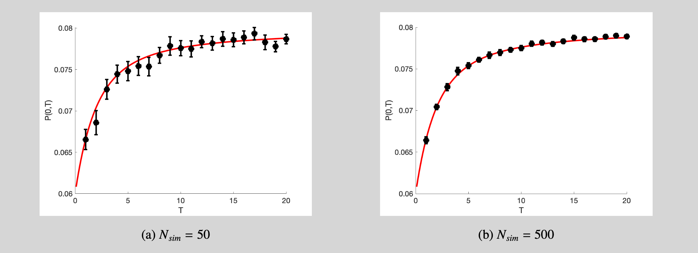
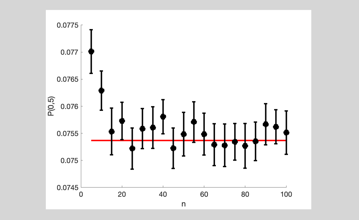
Visual evidence for this simulated approach is available in Figures 2–3. We have taken $r_0=6%$, $\theta=0.08$, $\kappa=0.86$, and $\sigma=0.01$. The (estimated) zero-coupon bond prices from \eqref{eq:approx} are converted into yields. Figure 2 shows that: (1) differences between simulated and exact yields are small, and (2) variability between simulated yields decreases when $N_{sim}$ increases from 50 to 500. The influence of $n$ is portrayed in Figure 3. In practice, we can use these kind of graphs to decide on suitable choices for $n$ and $N_{sim}$. Simply select a pair $(n,N_{sim})$ and verify whether the computed quantity is insensitive to changes therein.

Appendix

Recall $\Lambda(t) = \int_0^t e^{-\kappa s} ds = \frac{1}{\kappa}\left[ 1 - e^{-\kappa t} \right]$ and note how it implies \begin{equation} \begin{aligned} \int_x^T e^{-\kappa(s-x)} ds &= e^{\kappa x} \Big[ \Lambda(T) - \Lambda(x) \Big] = \tfrac{1}{\kappa} e^{\kappa x} \left[ e^{-\kappa x} - e^{-\kappa T}\right] \\ & = \Lambda(T-x). \end{aligned} \label{eq:MyINT} \tag{A1} \end{equation} The integral in this last equation will be used at several occasions in the derivations below. Using the expression for $r(t)$, we have $$ \begin{aligned} \int_t^T r(s) ds &= \int_t^T e^{-\kappa s} r(0) ds \\ & \quad + \int_t^T \int_0^s e^{-\kappa(s-x)} \kappa \theta dx ds + \int_t^T \int_0^s e^{-\kappa (s-x)}\sigma dW(x) ds \\ &=: I+II+III. \end{aligned} $$ We will develop these three contributions separately. Term $I$ is easiest. Using \eqref{eq:MyINT}, we find $$ I = \int_t^T e^{-\kappa s} r(0) ds = r(0) e^{-\kappa t} \int_t^T e^{ -\kappa(s-t) }ds = r(0) e^{-\kappa t} \Lambda(T-t). $$

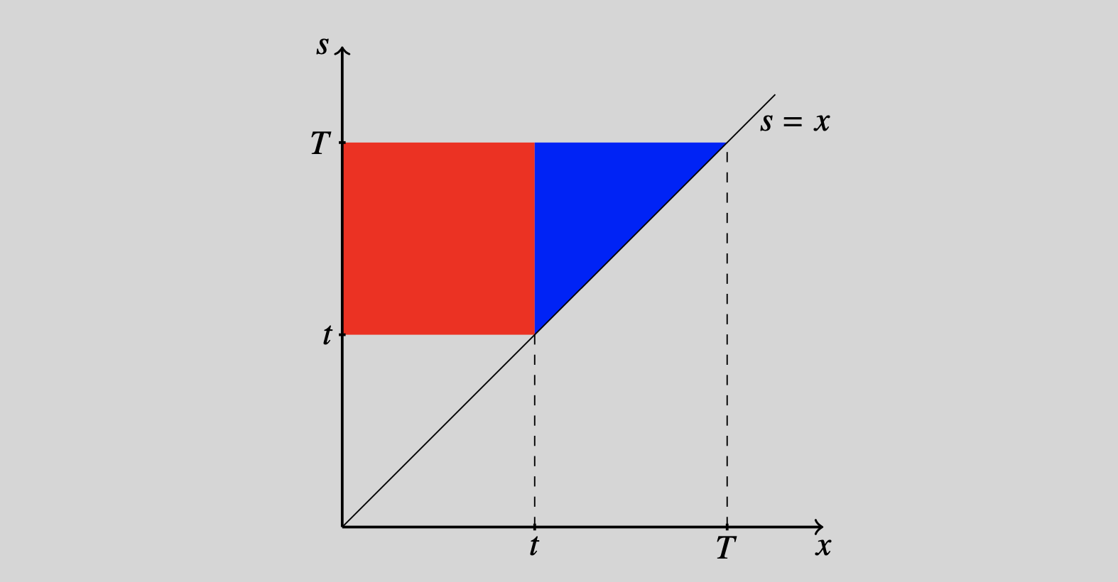
Term $II$ requires a change in the order of integration. Inspecting the area of integration in Figure 4, we arrive at the following integral relation $$ \begin{aligned} II &= \int_t^T \int_0^s e^{-\kappa(s-x)} \kappa \theta dx ds \\ &= \int_0^t \int_t^T e^{-\kappa(s-x)} \kappa \theta ds dx + \int_t^T \int_x^T e^{-\kappa(s-x)} \kappa \theta ds dx \\ &= \int_0^t \int_t^T e^{-\kappa(s-t+t-x)} \kappa \theta ds dx + \kappa \theta \int_t^T \Lambda(T-x) dx \\ &= \int_0^t e^{-\kappa(t-x)}\kappa \theta dx , \Lambda(T-t) + \kappa \theta \int_t^T \Lambda(T-x) dx. \end{aligned} $$ We apply exactly the same change in the order of integration to term $III$. The result is $$ \begin{aligned} III &= \int_t^T \int_0^s e^{-\kappa (s-x)}\sigma dW(x) ds \\ &= \int_0^t \int_t^T e^{-\kappa (s-x)}\sigma ds dW(x) + \int_t^T \int_x^T e^{-\kappa (s-x)}\sigma ds dW(x) \\ &= \int_0^t \int_t^T e^{-\kappa (s-t+t-x)}\sigma ds dW(x) + \sigma \int_t^T \Lambda(T-x)dW(x) \\ &= \int_0^t e^{-\kappa(t-x)} \sigma dW(x) , \Lambda(T-t) + \sigma \int_t^T \Lambda(T-x)dW(x). \end{aligned} $$ If terms $I$–$III$ are added together, then we see that $\int_x^T e^{-\kappa(s-x)} ds$ is an affine transformation of the prevailing short rate $r(t)$, i.e. $$ \begin{aligned} \int_t^T &r(s) ds \\ & = I+II+III \\ &= \left[ r(0) e^{-\kappa t} + \int_0^t e^{-\kappa(t-x)}\kappa \theta dx+\int_0^t e^{-\kappa(t-x)} \sigma dW(x) \right] \Lambda(T-t) \\ &\quad+ \kappa \theta \int_t^T \Lambda(T-x) dx+\sigma \int_t^T \Lambda(T-x)dW(x) \\ &= r(t) \Lambda(T-t)+\kappa \theta \int_t^T \Lambda(T-x) dx+\sigma \int_t^T \Lambda(T-x)dW(x). \end{aligned} $$ Conditional on all information up to time t, i.e. conditional on $\mathcal{F}_t$, the first two terms are deterministic. Moreover, since (1) increments of Brownian motions are independent of the current value and (2) stochastic integrals are normally distributed, we know that $ \left.\int_t^T r(s) ds\right| \mathcal{F}_t$ is normally distributed with mean $$ \begin{aligned} r(t) \Lambda(T-t) &+\kappa \theta \int_t^T \Lambda(T-x) dx \\ &= r(t) \Lambda(T-t)+\kappa \theta \int_0^{T-t} \Lambda(x) dx \\ &= r(t) \Lambda(T-t) + \theta\Big[(T-t) - \Lambda(T-t) \Big] \end{aligned} $$ and by Itô isometry a variance of $$ \begin{aligned} \sigma^2 \int_t^T &\big[ \Lambda(T-x) \big]^2 dx = \sigma^2 \int_0^{T-t} \big[ \Lambda(x) \big]^2 dx \\ &= \tfrac{\sigma^2}{\kappa^2} \int_0^{T-t} \left( 1-2 e^{-\kappa x} + e^{-2\kappa x} \right) dx \\ &= \tfrac{\sigma^2}{\kappa^2} \left[ (T-t) -2 \int_0^{T-t} e^{-\kappa x} dx + \tfrac{1}{2} \int_0^{2(T-t)} e^{-\kappa x} dx \right] \\ &= \tfrac{\sigma^2}{\kappa^2} \left[ (T-t) -2 \Lambda(T-t) + \tfrac{1}{2} \Lambda\Big(2(T-t) \Big) \right]. \end{aligned} $$

References

N. H. Bingham and R. Kiesel (2004), Risk-neutral Valuation, Springer Finance

D. Filipović (2009), Term-structure Models, Springer Finance

T. Mikosch (1998), Elementary Stochastic Calculus with Finance in View, World Scientific