Which computational language to choose?

Short intro

Let us compare the performance of C++, Matlab, Python and R when performing typical econometrical/statistical tasks. The word ‘typical’ is quite ambiguous since computational requirements can vary substantially between subfields. As such, I will consider a setting that is standard yet also computationally demanding: bootstrap inference on the Durbin-Watson test statistic. This setting is easy to understand and the computational performance of the programming languages is probably representative for a wide range of Monte Carlo (MC) simulations. MC simulations are very often needed in research when relying on frequentist statistics.

The Durbin-Watson test statistic

Consider a standard multivariate regression model $y_t^{} = \mathbf{x}_t’ \boldsymbol \beta + u_t^{}$ for $t = 1, 2, . . . , T$. The presence of serial correlation in $u_t$ will render standard ordinary least squares (OLS) inference invalid. The Durbin-Watson test statistic was one of the first test statistics to test for the presence of serial correlation.¹ It is computed as follows:

1. Calculate the OLS estimator $\widehat{\boldsymbol \beta}=(\mathbf{X}’\mathbf{X})^{-1} \mathbf{X}’\mathbf{y}$.
2. Obtain the residuals $\widehat{u}_t=y_t- \mathbf{x}_t’\widehat{\boldsymbol \beta}$ for $t = 1, 2, . . . , T$.
3. The Durbin-Watson test statisic is now computed as $DW= \frac{\sum_{t=2}^T \left(\widehat{u}_t-\widehat{u}_{t-1}\right)^2 }{\sum_{t=1}^T \widehat{u}_t^2}$.

Simple algebraic manipulations show that the Durbin-Watson statistic can be expressed in terms of the first order sample autocorrelation $\widehat{\rho}= \frac{\sum_{t=2}^T \widehat{u}_t\widehat{u}_{t-1} }{\sum_{t=1}^T \widehat{u}_t^2}$, namely $DW=2(1-\widehat{\rho})-\frac{\widehat{u}_1^2+\widehat{u}_T^2}{\sum_{t=1}^T \widehat{u}_t^2}$. Based on this result we would expect outcomes close to the value 2 if first order autocorrelation is absent. Values different from 2 indicate serial correlation. Using the Durbin-Watson statistic to carry out a formal hypothesis test is more complicated because its (asymptotic) distribution is difficult to derive. This motivates the use of a bootstrap approach.² The specific steps are:

1. Estimate $\boldsymbol \beta$ by OLS and compute the residual series ${\widehat{u}_t }$ as well as the Durbin-Watson statistic $DW$.
2. Compute $\widehat{\rho}$ (see the definition above) and $\widehat{\varepsilon,}_t=\widehat{u}_t- \widehat{\rho} \widehat{u}_{t-1}$ for $t=2,3,\ldots,T$.
3. Draw bootstrap errors $\varepsilon_t^\star$ by resampling with replacement from $\{\widehat{\varepsilon}_2,\widehat{\varepsilon,}_3,\ldots,\widehat{\varepsilon,}_T \}$. Store these in the vector $\boldsymbol \varepsilon^\star=[\varepsilon_1^\star,\varepsilon_2^\star,\ldots,\varepsilon_T^\star]’ $.
4. Set $\mathbf{u}^\star=\boldsymbol \varepsilon^\star$ (to impose the null hypothesis in the bootstrap sample), construct the bootstrap sample $\mathbf{y}^\star=\mathbf{X}\widehat{\boldsymbol \beta}+\mathbf{u}^\star$, and compute the DW statistic from $\mathbf{y}^\star$.
5. Repeat steps 3-4 $B$ times and store these outcomes in a list $\left\{ DW_b^\star \right\}_{b=1}^B$.
6. For a given significance level $\alpha$, we define $q_{\alpha/2}^\star$ and $q_{1-\alpha/2}^\star$ as the $\alpha/2$ and $1-\alpha/2$ empirical quantiles of $\left\{ DW_b^\star \right\}_{b=1}^B$. We reject the null hypothesis of no serial correlation if either $DW < q_{\alpha/2}^\star$ or if $DW>q_{1-\alpha/2}^\star$.

The simulation setting

We consider a simple simulation setting to compare the different programming environments, namely

$$ \begin{aligned} y_t &= \mathbf{x}_t’\boldsymbol{\beta}+u_t \\\ u_t &= \rho u_{t-1}+\varepsilon_t, \qquad \qquad t=1,2,\ldots,T, \end{aligned} $$

where $T=\{100,250,500\}$. The fixed regressor matrix $\mathbf{X}$ contains a column of ones and a column that repeats the sequence $0,1,0,-1$ (orthogonal design). The error terms ${\epsilon_t}$ are standard normal and a presample of 50 observations is used to remove the influence of the initial values. We set $\boldsymbol \beta=[1,2]’ $ and vary the value for $\rho$ over the grid $[0,0.025,\ldots,0.5]’ $ (21 grid points). The resulting power curves are depicted in Figure 1. Overall, we use 1000 Monte Carlo replications where each replication uses $B=499$ bootstrap resamples.

Results and discussion

Simulations are performed on a Macbook with a 2.6 GHz Intel Core i5 processor. I used serial computing. The computational times are reported in Table 1.

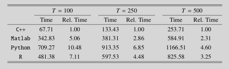
The conclusions from this table are unambiguous. The C++ implementation is significantly faster than the scientific programming environments of Matlab and R. However, this should be balanced against the fact that the programming itself is much easier/faster in the user-friendly environments offered by either of these languages. The results do not promote the use of Python. The computational times are longest and coding is less comfortable because matrix algebra requires an additional library (such as numpy). My conclusions are qualitatively the same as those in Borağan Aruoba and Fernández-Villaverde (2015).³

References