The GARCH(1,1) model and its extensions

The GARCH(1,1) model was proposed in Bollerslev (1986). The early publication date of this paper might give the impression that the model is somewhat outdated. Regardless of whether or not this last sentence is true, there are still two important reasons to discuss this model: (1) a discussion of the GARCH(1,1) model facilitates the understanding of more complex univariate GARCH specifications, and (2) many multivariate GARCH models follow a similar methodology. The GARCH(1,1) specification reads:

\begin{equation} \begin{aligned} y_t &= \sigma_t \eta_t,\qquad\qquad\qquad\qquad \eta_t \stackrel{i.i.d.}{\sim} (0,1), \\ \sigma_t^2 &= \omega + \alpha y_{t-1}^2 + \beta \sigma_{t-1}^2, \end{aligned} \tag{1} \label{eq:GARCHspec} \end{equation} where $\eta_t \stackrel{i.i.d.}{\sim} (0,1)$ is shorthand indicating an independent and identically distributed series ${\eta_t}$ with mean $\mathbb{E}[\eta_t]=0$ and variance $\mathbb{V}\mathrm{ar}[\eta_t]=1$. The unknown parameters in the model are $\omega>0$, $\alpha\geq 0$, and $\beta\geq 0$. For convenience, we stack all parameters in the $(3\times 1)$ vector $\boldsymbol{\theta}=(\omega,\alpha,\beta)^\prime$.

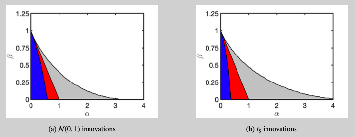
The GARCH(1,1) model defines the volatility process ${\sigma_t^2}$ recursively. To see this, we note that $y_{t-1}^2=\sigma_{t-1}^2 \eta_{t-1}^2$ and rewrite the volatility recursion in \eqref{eq:GARCHspec} as $\sigma_t^2=\omega+\big(\alpha \eta_{t-1}^2+ \beta \big)\sigma_{t-1}^2$. By repeated substitution, the volatility process $\sigma_t^2$ is subsequently rewritten as \begin{equation} \begin{aligned} \sigma_t^2 &= \omega + \big( \alpha \eta_{t-1}^2+ \beta \big) \sigma_{t-1}^2 \\ &= \omega + \big( \alpha \eta_{t-1}^2+ \beta \big) \Bigg( \omega + \big( \alpha \eta_{t-2}^2+ \beta \big) \sigma_{t-2}^2 \Bigg) \\ &= \ldots = \omega \left(1 + \sum_{j=1}^\infty \prod_{i=1}^j \big( \alpha \eta_{t-i}^2+ \beta \big) \right), \end{aligned} \tag{2} \label{eq:sigma2expr} \end{equation} whenever the infinite sum $ \sum_{j=1}^\infty \prod_{i=1}^j \big( \alpha \eta_{t-i}^2+ \beta \big)$ converges in a statistically meaningful sense. A sufficient condition for convergence (see, e.g. section 2.2 in Francq and Zakoian (2019)) is \begin{equation} \mathbb{E}\Big[\log(\alpha \eta_t^2 + \beta) \Big] < 0. \tag{3} \label{eq:stationaritycondition} \end{equation} This convergence criterion depends on: the parameter $\alpha$, the parameter $\beta$, and the distribution of $\eta_t$. Overall, if condition \eqref{eq:stationaritycondition} is fulfilled, then the GARCH(1,1) process is uniquely defined and it will be strictly stationary.¹ More stringent parameter conditions are needed to guarantee finite higher moments. An illustration is provided in Figure 1.

Statistical Properties of the GARCH(1,1) Process

We first investigate the covariance structure of the levels of a GARCH(1,1) process. Let $\mathcal{F}_t=\sigma(y_u; u\leq t)$ denote the $\sigma$-algebra containing all information up to and including time $t$. Since $\sigma_t$ depends solely on observations prior to time $t$, the law of iterated expectations provides

\begin{equation} \mathbb{E}[y_t] = \mathbb{E}\Big[ \mathbb{E}[y_t \mathcal{F}_{t-1}] \Big]= \mathbb{E}\Big[ \sigma_{t} \mathbb{E}[ \eta_t \mathcal{F}_{t-1}] \Big]=0. \end{equation}

Similarly, since $\mathbb{V}\text{ar}[\eta_t]=\mathbb{E}[\eta_t^2]=1$, we have $\mathbb{V}\text{ar}[y_t]=\mathbb{E}[\sigma_t^2]$. This last expectation is rather easily computed using \eqref{eq:sigma2expr}. Indeed, the i.i.d. property of the series ${\eta_t}$ combined with $\mathbb{E}[a(\eta_{t-i};\boldsymbol \theta)]=\alpha+\beta$ (for any $i\in\mathbb{Z}$) provides

\begin{equation} \begin{aligned} \mathbb{E}[\sigma_t^2] &= \omega \left(1 + \sum_{i=1}^\infty \mathbb{E}\big[a(\eta_{t-1}^2;\boldsymbol \theta)\big] \cdots \mathbb{E}\big[ a(\eta_{t-i}^2;\boldsymbol \theta) \big] \right) \\ &= \omega \left(1 + \sum_{i=1}^\infty (\alpha+\beta)^i \right)= \frac{\omega}{1-\alpha-\beta}, \end{aligned} \label{eq:expsigma2} \end{equation}

assuming that the geometric series converges, i.e. assuming $\alpha+\beta<1$.² The covariance structure of the levels of the GARCH(1,1) process is now clear. If $\alpha+\beta<1$, then $\mathbb{V}\text{ar}[y_t]=\omega/(1-\alpha-\beta)$ and $$ \begin{aligned} \mathbb{C}\text{ov}[y_t, y_{t-j}] &= \mathbb{E}[y_t y_{t-j}] \\ &= \mathbb{E}\big[ \sigma_t y_{t-j} \mathbb{E}[\eta_t|\mathcal{F}_{t-1}] \big] = 0,\qquad\text{for }j=1,2,\ldots. \end{aligned} $$ Overall, this shows that the levels of a GARCH(1,1) process have an unconditional variance of $\mathbb{V}\text{ar}[y_t]=\omega/(1-\alpha-\beta)$ and do not exhibit autocorrelation.

Because the GARCH(1,1) process is designed to model volatility (the second moment), all interesting properties are related to the covariance structure of $y_t^2$. The kurtosis of $y_t$, $\kappa_y = \mathbb{E}[y_t^4]/\big(\mathbb{V}\text{ar}[y_t]\big)^2$, is computed along the way. As full derivations are somewhat tedious, we relegate all details to the appendix. The two most important findings are:

1. If $\lambda = \mathbb{E}\big[(\alpha \eta_t^2+ \beta)^2\big] <1$, then $\kappa_y$ exists. Denoting the kurtosis of the innovations by $\kappa_\eta = \mathbb{E}[\eta_t^4]$, its mathematical expression is $$ \begin{aligned} \kappa_y &= \left( 1 + \frac{\mathbb{V}\mathrm{ar}[\alpha\eta_t^2+\beta]}{1-\lambda} \right) \kappa_\eta \\ &= \frac{1-(\alpha+\beta)^2}{1-(\alpha+\beta)^2 - \alpha^2(\kappa_\eta -1)} \kappa_\eta. \end{aligned} $$ The recursive nature of the volatility process thus causes the kurtosis of the GARCH(1,1) process to exceed the kurtosis of its innovations.
2. The autocorrelations of the squares of a GARCH(1,1) process decay geometrically, i.e. $\rho_k = \mathbb{C}\mathrm{or}[y_t^2,y_{t-k}^2] = \rho_1(\boldsymbol \theta) (\alpha+\beta)^{k-1}$ where $\rho_1(\boldsymbol \theta)$ is a function of the parameters $\alpha$ and $\beta$ but not of $k$.

Estimation

GARCH(1,1) models are frequently estimated by conditional Gaussian quasi-maximum likelihood. The second part of this terminology, Gaussian quasi-maximum likelihood, refers to the gaussianity assumption we place upon the distribution of ${\eta_t}$. That is, our likelihood derivation simply assumes $\eta_t \stackrel{i.i.d.}{\sim} \mathcal{N}(0,1)$ even when the true innovation density is different. Our inference is conditional because we select some fixed initial values for $y_0$ and $\sigma_0^2$ ourselves. The precise estimation steps are enumerated below.

Step 1. Set initial values for $y_0$ and $\tilde\sigma_0^2$. A common choice is the unconditional variance for the volatility, $\tilde\sigma_0^2=\omega/(1-\alpha-\beta)$, and $y_0=\tilde\sigma_0$.

Step 2. Given the observations $y_1,\ldots,y_T$ and a parameter vector $\boldsymbol \theta=(\omega,\alpha,\beta)$’, we recursively compute $\{\tilde\sigma_t^2(\boldsymbol \theta)\}_{1\leq t\leq T}$ using \begin{equation} \tilde\sigma_t^2(\boldsymbol \theta) = \tilde\sigma_t^2 = \omega + \alpha y_{t-1}^2 + \beta \tilde\sigma_{t-1}^2. \label{eq:ApproximateVolatility} \end{equation} The value of $\tilde\sigma_t^2(\boldsymbol \theta)$ is determined by all observations up to and including time $t-1$.

Step 3. Approximating the volatility process $\sigma_t^2$ by $\tilde\sigma_t^2(\boldsymbol \theta) $ and recalling the gaussianity assumption on the innovations, we have $y_t|y_{t-1},\ldots,y_1\sim \mathcal{N}(0,\tilde\sigma_t^2)$. The quasi-likelihood is thus $$ L_T(\boldsymbol \theta) = \prod_{i=1}^T \frac{1}{\sqrt{2\pi \tilde\sigma_t^2(\boldsymbol \theta)}} \exp\left( - \frac{y_t^2}{2 \tilde\sigma_t^2(\boldsymbol \theta)} \right). $$ The maximisation of the quasi-likelihood is identical to the minimisation of $$ \bar\ell_T(\boldsymbol \theta) = \frac{1}{T} \sum_{t=1}^T \tilde\ell_t(\boldsymbol \theta),\text{ where }\tilde\ell_t(\boldsymbol \theta) = \frac{y_t^2}{\tilde\sigma_t^2(\boldsymbol \theta)} + \log\big( \tilde\sigma_t^2(\boldsymbol \theta) \big). $$ This latter representation is more suitable when numerically solving this nonlinear optimisation problem. Stationarity conditions can be imposed during estimation.

Parameter Inference

Under suitable regularity conditions, the quasi-maximum likelihood estimator (QMLE) $\hat{\boldsymbol \theta}_T$ is asymptotically normally distributes:

\begin{equation} \sqrt{T} \big( \hat{\boldsymbol \theta}_T - \boldsymbol\theta \big) \stackrel{D}{\rightarrow} \mathcal{N}\Big( \boldsymbol 0,(\kappa_\eta-1) \mathbf{J}^{-1}\Big) \qquad\text{as}\qquad T\to\infty, \label{eq:AsymptoticDistribution} \tag{4} \end{equation}

where $\kappa_\eta=\mathbb{E}[\eta_t^4]$ (the kurtosis of the innovations) and $\boldsymbol J = \mathbb{E}\left[\frac{\partial^2 \ell_t}{\partial \boldsymbol \theta \partial \boldsymbol \theta’}\right]$ with $\ell_t=\frac{y_t^2}{\sigma_t^2(\boldsymbol \theta)} + \log\big( \sigma_t^2(\boldsymbol \theta) \big)$. The full details of the derivation can be found in Chapter 7 of Francq and Zakoian (2019). Broadly speaking, the proof consists of three steps:

1. Establishing that $\{\tilde{\sigma}_t^2(\boldsymbol \theta)\}$ is close to $\{\sigma_t^2(\boldsymbol \theta)\}$. That is, the initialisation of $y_0$ and $\tilde\sigma_0^2$ in Step 1 should have a negligible influence asymptotically. This is expected to hold because stationarity requirements such as $\alpha+\beta<1$ imply both $\alpha<1$ and $\beta<1$. Looking at the recursion $\sigma_t^2 = \omega + \alpha y_{t-1}^2 + \beta \sigma_{t-1}^2$, we see that the impact of the initialisation will decay rapidly in $t$.

2. Proving consistency of the QMLE, i.e. proving $\hat{\boldsymbol \theta}_T \stackrel{P}{\to} \boldsymbol\theta$ as $T\to\infty$. This is the most difficult step because it requires (uniform) convergence of the objective function to a limiting criterion function with a unique optimum.

3. As in the usual likelihood framework, a mean-value expansion of the gradient of the quasi-likelihood around $\boldsymbol \theta$ provides the asymptotic distribution.

The result in \eqref{eq:AsymptoticDistribution} is rather easily used for (asymptotically) valid inference because consistent estimators for $\boldsymbol J$ and $\kappa_\eta$ are readily available. A consistent estimator for $\boldsymbol J$ is the Hessian of the average quasi-likelihood evaluated at $\hat{\boldsymbol\theta}_T$:

$$ \hat{\boldsymbol J}_T = \frac{\partial^2\bar\ell_T(\hat{\boldsymbol\theta}_T)}{\partial \boldsymbol \theta \partial \boldsymbol \theta’} = \frac{1}{T} \sum_{t=1}^T\frac{\partial \tilde\ell_t(\hat{\boldsymbol\theta}_T)}{\partial \boldsymbol \theta \partial \boldsymbol \theta’}. $$

This Hessian matrix is usually immediately available from the numerical optimiser. A subsequent run of the volatility recursions at the estimated parameters gives estimated innovations $\hat\eta_t = y_t/ \tilde\sigma_t(\hat{\boldsymbol \theta}_T)$ ($t=1,\ldots,T$). The sample kurtosis of these estimated innovations consistently estimates $\kappa_\eta$.

Illustration

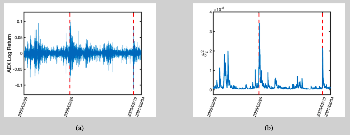
We illustrate the model using log-returns from the AEX index for 2000/08/08 until 2021/08/04. The $T=5400$ observations are visualised in Figure 2(a).³ The Gaussian quasi-maximum likelihood estimates are: $\hat\omega=2.33\times 10^{-6}$, $\hat\alpha=0.109$, and $\hat\beta=0.876$. With these parameter estimates, we can initialise the estimated volatility process as $\hat\sigma_0=\hat\omega/(1-\hat\alpha-\hat\beta)$ and iterate through $\hat\sigma_t = \hat\omega + \hat\alpha y_{t-1}^2+\hat\beta \hat\sigma_{t-1}^2$ to approximate the volatility over time (Figure 2(b)). Clearly, the estimated volatility peaks during the Global Financial crisis (2008/09/29) and around the introduction of the preventive Coronavirus regulations in the Netherlands (2020/03/12). The ability to model the conditional volatility as time-varying and thereby capture volatility clusters is one of the successes of GARCH modelling.

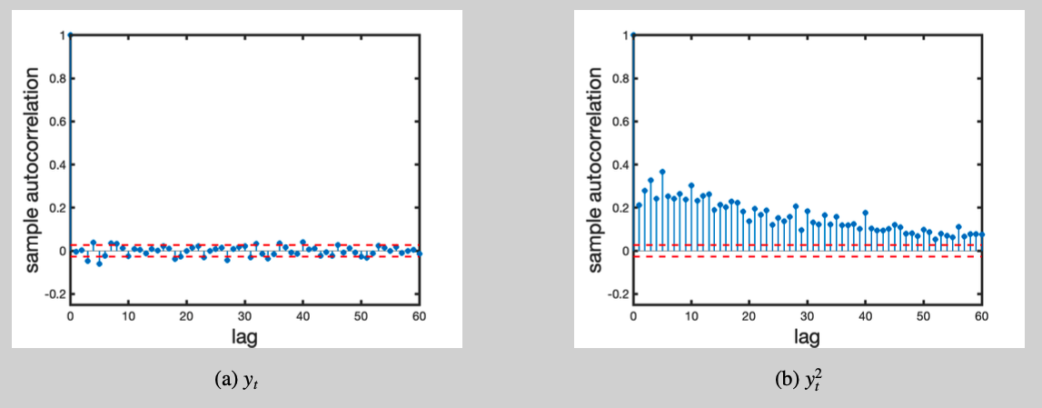
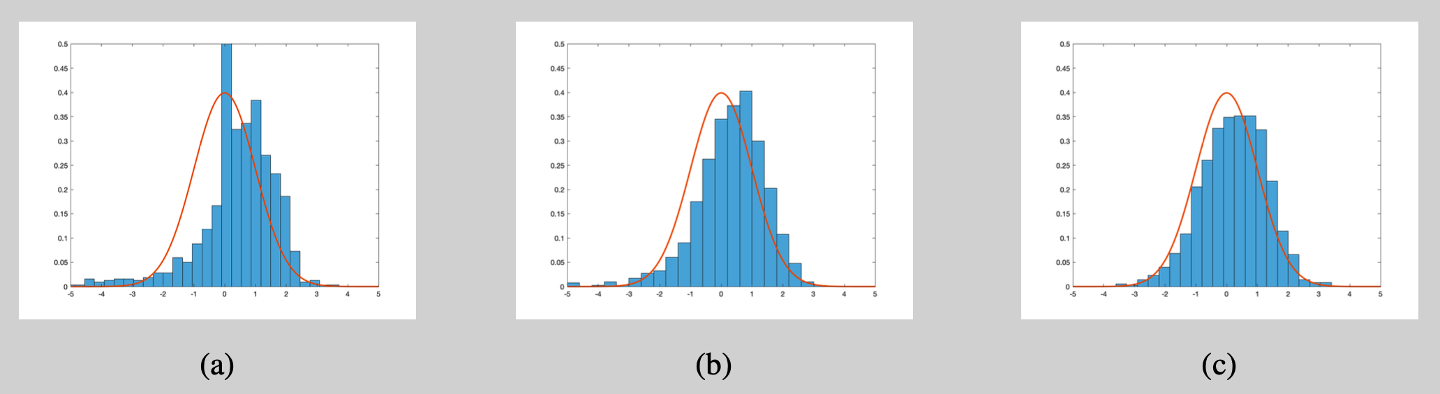
This empirical example can also demonstrate how the GARCH(1,1) model can successfully replicate other stylised facts from financial data. First, we look at the autocorrelation function (ACF) of both $y_t$ and $y_t^2$ (Figure 3). The absence of autocorrelation in $y_t$ and the slow decay of the autocorrelations in $y_t^2$ align well with the theoretical properties of the GARCH(1,1) model. Second, some statistical characteristics of the innovations can be explored through the residuals $\hat\eta_t = y_t/\hat\sigma_t$ ($t=1,\ldots,T$). The sample kurtosis of the log-returns and residuals are $\hat\kappa_y = 10.55$ and $\hat\kappa_\eta=4.10$, respectively. The mismatch between these numbers indicates that the recursive structure of the GARCH(1,1) model should amplify the tails of the innovation distribution considerably.

Extensions

The main idea behind the GARCH(1,1) process, i.e. the volatility update based on past volatility and past realisations, can be generalised beyond the current GARCH(1,1) setting. A non-exhaustive list of generalisations is presented below.

1. The digits in the GARCH(1,1) specification indicate the number of lags of the volatility and squared observations influencing $\sigma_t^2$, respectively. That is, the general GARCH($p$,$q$) process reads \begin{equation} \begin{aligned} y_t &= \sigma_t \eta_t,\qquad\qquad\qquad\qquad\qquad\qquad \eta_t \stackrel{i.i.d.}{\sim} (0,1). \\ \sigma_t^2 &= \omega + \sum_{i=1}^q \alpha y_{t-i}^2 + \sum_{j=1}^p \beta_j \sigma_{t-j}^2, \end{aligned} \label{eq:GARCHpq} \end{equation} Clearly, the GARCH(1,1) process is simply a GARCH($p$,$q$) process with $p=q=1$. The additional lags in the GARCH($p$,$q$) allow for a better fit to the data while keeping the developed intuition from the GARCH(1,1) model intact. The paper by P. R. Hansen and A. Lunde – A Forecast Comparison of Volatility Models: Does Anything Beat a GARCH(1,1)? – probably explains why the GARCH(1,1) model has become somewhat of a benchmark.

2. The volatility of the GARCH(1,1) model does not distinguish positive and negative past returns. That is, only $y_{t-1}^2$ (note the square) affects the volatility. However, if volatility is interpreted as riskiness, then we might expect a past negative return to have a larger impact on volatility than a past positive return. A Threshold GARCH (TGARCH) model allows for this leverage effect. Defining $y_t^+=\max(y_t,0)$ and $y_t^- = \max(-y_t,0)$, the TGARCH(1,1) specification is \begin{equation} \begin{aligned} y_t &= \sigma_t \eta_t,\qquad\qquad\qquad\qquad\qquad\qquad\qquad \eta_t \stackrel{i.i.d.}{\sim} (0,1). \\ \sigma_t^2 &= \omega + \alpha_{1,+} y_{t-1}^+ + \alpha_{1,-} y_{t-1}^- + \beta \sigma_{t-1}^2, \end{aligned} \label{eq:TGARCHspec} \end{equation}

3. Multivariate extensions of the GARCH(1,1) model are needed if multiple return series are to be investigated simultaneously. Let $\mathbf{y}_t\in \mathbb{R}^m$ denote the $m$-dimensional return vector at time $t$. There are two popular modelling strategies. The first strategy is a direct multivariate generalisation of \eqref{eq:GARCHspec}. That is, we let $\boldsymbol \eta_t\stackrel{i.i.d.}{\sim} (\boldsymbol 0, \boldsymbol{I}_m)$ denote an i.i.d. sequence of $m$-dimensional innovations with mean vector $\boldsymbol 0$ and an identity matrix as covariance matrix. The model assumes $$ \mathbf{y}_t = \boldsymbol H_t^{1/2} \boldsymbol\eta_t, $$ with $\boldsymbol H_t \in \mathbb{R}^{m\times m}$ following a recursive structure. Different recursive structures will lead to different multivariate GARCH (MGARCH) models. One example is the BEKK-GARCH(1,1), $$ \boldsymbol H_t = \boldsymbol\Omega + \boldsymbol A \boldsymbol{y}_{t-1} \boldsymbol{y}_{t-1}’ \boldsymbol A’ + \boldsymbol B \boldsymbol H_{t-1} \boldsymbol B’, $$ as introduced in Engle and Kroner (1995).⁴ The similarities to the GARCH(1,1) specification should be evident as the outer product $\boldsymbol{y}_{t-1} \boldsymbol{y}_{t-1}^\prime$ and conditional covariance matrix $\boldsymbol H_t$ are the natural multivariate extensions to respectively $y_{t-1}^2$ and $\sigma_t^2$ of the GARCH(1,1) model. The main issue with this class of MGARCH models is parameter interpretability and the difficulties in ensuring stationarity and positive-definiteness of $\boldsymbol H_t$.

   The second strategy, the so-called Cholesky GARCH models, starts from a collection of $m$ univariate processes. For $i=1,\ldots,m$, we thus consider \begin{equation} \begin{aligned} v_{it} &= \sqrt{g_{it}} \eta_{it},\\ g_{it} &= \omega_i + \alpha_i v_{i,t-1}^2 + \beta_i g_{i,t-1}, \end{aligned} \label{eq:CholeskyGARCHspec} \end{equation} or in vector form as $\boldsymbol v_{t} = \boldsymbol G_t^{1/2} \boldsymbol \eta_t$ after defining $\boldsymbol{v}_t = (v_{1t},\ldots,v_{mt})^\prime$ and $\boldsymbol{G}_t = \text{diag}(g_{1t},\ldots, g_{mt})$. A lower unitriangular matrix $\boldsymbol L$, that is a matrix of the form $$ \boldsymbol L = \begin{bmatrix} 1 \\ l_{2,1} & 1 \\ \vdots & \ddots & \ddots \\ l_{m-1,1} & & \ddots & 1\\ l_{m,1} & l_{m,2} & \cdots & l_{m,m-1} & 1
   \end{bmatrix}, $$ subsequently connects the univarariate GARCH(1,1) process with the return series through $\boldsymbol y_t = \boldsymbol L \boldsymbol v_t = \boldsymbol L \boldsymbol G_t^{1/2} \boldsymbol \eta_t$.⁵ The advantages of Cholesky GARCH are: (1) the conditional variance $\boldsymbol L \boldsymbol{G}_t \boldsymbol{L}^\prime$ is positive-definite by construction, and (2) the elements in $\boldsymbol L^{-1}$ are interpretable as conditional betas. The main disadvantage of Cholesky GARCH is that the model is not invariant to changes in the ordering of the return series.

A Computation Comparison

Finally, we conduct a Monte Carlo simulation to compare computational speeds across Matlab, Python and R. The computational tasks are: (1) generating a GARCH(1,1) process with standard Gaussian innovations and $(\omega,\alpha,\beta)^{\prime}= (0.1, 0.05, 0.8)^{\prime}$ (ensuring stationarity), (2) estimating the parameters by conditional quasi-maximum likelihood using the generated data series, and (3) computing the asymptotically valid t-statistic based on the limiting distribution in \eqref{eq:AsymptoticDistribution}. We use $N_{sim}=1000$ Monte Carlo replications. To see the code, click the corresponding button at the top of this blog.

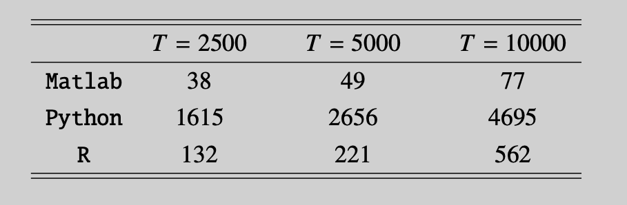
The results are shown in Figure 4 and Table 1. We make the following two observations:

1. Theoretically, the standardised statistics converge in distribution to a standard normal as $n\to\infty$. The finite sample distribution of the test statistics (Figure 4) indeed seems to approach the $\mathcal{N}(0,1)$ distribution but truly large sample sizes are needed.
2. The Matlab and Python implementation are fastest and slowest, respectively. The same ranking was also observed in this previous post. The overall speed of the implementation is probably determined by the speed of for-loops (to recursively compute the volatility process) and the numerical optimiser (fmincon() for Matlab, the minimize() function from scipy for Python, and optim() for R). The good performance of Matlab is thus perhaps unsurprising. Its for-loops are known to be quick and fmincon() is a pretty robust nonlinear optimisation routine.⁶

Appendix

Calculating $\mathbb{E}[y_t^4]$

By the law of iterated expectations, we have $\mathbb{E}[y_t^4]= \mathbb{E}[\sigma_t^4] \mathbb{E}[\eta_t^4]$. Clearly, $\mathbb{E}[\eta_t^4]$ is implied by the distributional assumption on $\eta_t$ and we only need to calculate $\mathbb{E}[\sigma_t^4]$. Using \eqref{eq:sigma2expr}, we find \begin{equation} \begin{aligned} \mathbb{E}\big[\sigma_t^4\big] &= \mathbb{E}\left[ \omega^2 \left(1 + \sum_{j=1}^\infty \prod_{i=1}^j \big( \alpha \eta_{t-i}^2+ \beta \big) \right)^2 \right] \\ &= \omega^2 \Bigg( 1 + 2 \sum_{j=1}^\infty \mathbb{E}\Bigg[ \prod_{i=1}^j \big( \alpha \eta_{t-i}^2+ \beta \big) \Bigg] \\ &\qquad\qquad+ \sum_{j=1}^\infty \sum_{k=1}^\infty \mathbb{E}\Bigg[\prod_{i=1}^j \prod_{l=1}^k \big( \alpha \eta_{t-i}^2+ \beta \big) \big( \alpha \eta_{t-l}^2+ \beta \big) \Bigg] \Bigg). \end{aligned} \label{eq:expsigma4} \end{equation} For brevity, we define $\zeta = \mathbb{E}\big[\alpha \eta_t^2+ \beta\big]=\alpha+\beta$ and $\lambda = \mathbb{E}\big[(\alpha \eta_t^2+ \beta)^2\big]=\alpha^2 \mathbb{E}\big[\eta_t^4 \big]+2\alpha\beta + \beta^2$. Standard results on geometric series imply \begin{equation} \begin{aligned} \mathbb{E}\big[\sigma_t^4\big] &= \omega^2 \left( 1 + 2 \sum_{j=1}^\infty \zeta^j + \sum_{j=1}^\infty \sum_{k=1}^\infty \lambda^{\min(j,k)} \zeta^{\max(j,k)-\min(j,k)} \right) \\ &= \omega^2 \left( 1 + 2 \sum_{j=1}^\infty \zeta^j + \sum_{j=1}^\infty \lambda^j + 2 \sum_{j=1}^\infty \sum_{k=j+1}^\infty \lambda^j \zeta^{k-j} \right) \\ &= \omega^2 \left( 1 + \frac{2\zeta}{1-\zeta}+ \frac{\lambda}{1-\lambda}+ \frac{2 \zeta}{1-\zeta} \frac{\lambda}{1-\lambda} \right) \\ &= \omega^2 \left( \frac{1}{1-\lambda} + \frac{2\zeta}{(1-\zeta)(1-\lambda)} \right) = \omega^2 \frac{1+\zeta}{(1-\zeta)(1-\lambda)} \\ &= \big( \mathbb{E}[\sigma_t^2] \big)^2 \frac{1-\zeta^2}{1-\lambda} = \big( \mathbb{E}[\sigma_t^2] \big)^2 \left( 1 + \frac{\mathbb{V}\mathrm{ar}[\alpha\eta_t^2+\beta]}{1-\lambda} \right) , \end{aligned} \tag{5} \label{eq:sigmat4} \end{equation} where the convergence of the geometric series requires $\lambda<1$. We also used $\mathbb{E}[\sigma_t^2] = \omega/(1-\alpha-\beta) = \omega/(1-\zeta)$ and $\mathbb{V}\mathrm{ar}[\alpha\eta_t^2+\beta]=\lambda-\zeta^2$.

Kurtosis

For any random variable $X$, its kurtosis is defined as its standardised fourth moment $$ \kappa_X = \mathbb{E}\left[\left(\frac{X-\mu}{\sqrt{\mathbb{V}\mathrm{ar}[X]}}\right)^4\right] . $$ Clearly, we have $\kappa_\eta=\mathbb{E}[\eta_t^4]$ and $\kappa_y=\mathbb{E}[y_t^4]/\big( \mathbb{E}[y_t^2]\big)^2$. The derivations in \eqref{eq:sigmat4} directly imply $$ \kappa_y = \frac{\mathbb{E}[y_t^4]}{\big( \mathbb{E}[y_t^2]\big)^2} = \frac{\mathbb{E}[\sigma_t^4]}{\big( \mathbb{E}[\sigma_t^2]\big)^2} , \mathbb{E}[\eta_t^4] = \left( 1 + \frac{\mathbb{V}\mathrm{ar}[\alpha\eta_t^2+\beta]}{1-\lambda} \right) \kappa_\eta. $$ As $0<\lambda<1$ (the upper bound is needed to guarantee the existence of $\mathbb{E}[y_t^4]$), this formula stresses the fact that $\kappa_y\geq \kappa_\eta$. The marginal distribution of $y_t$ thus has thicker tails than the distribution of the innovations. Using $\mathbb{V}\mathrm{ar}[\alpha\eta_t^2+\beta]=\alpha^2(\kappa_\eta-1)$ and $\lambda=(\alpha+\beta)^2 + \alpha^2(\kappa_\eta -1)$, the expression for $\kappa_y$ in terms of $\alpha$ and $\beta$ reads $$ \kappa_y = \frac{1-(\alpha+\beta)^2}{1-(\alpha+\beta)^2 - \alpha^2(\kappa_\eta -1)} \kappa_\eta. $$

Autocorrelations of the Squares of a GARCH(1,1) Process

For any $k>1$, using stationarity, the $k$^th autocorrelation of the square of a GARCH(1,1) process is \begin{equation} \begin{aligned} \rho_k &= \mathbb{C}\mathrm{or}[y_t^2,y_{t-k}^2] = \frac{\mathbb{C}\mathrm{ov}[y_t^2,y_{t-k}^2]}{\sqrt{\mathbb{V}\mathrm{ar}[y_t^2] , \mathbb{V}\mathrm{ar}[y_{t-k}^2] }} \\ &= \frac{\mathbb{C}\mathrm{ov}[y_t^2,y_{t-k}^2]}{\mathbb{V}\mathrm{ar}[y_t^2] } = \frac{\mathbb{E}[y_t^2 y_{t-k}^2] - \big( \mathbb{E}[y_t^2] \big)^2 }{ \mathbb{E}[y_t^4] - \big( \mathbb{E}[y_t^2] \big)^2 }. \end{aligned} \label{eq:autocorrelationcoef} \tag{6} \end{equation} Having derived $ \mathbb{E}[\sigma_t^4]$ in \eqref{eq:sigmat4}, the denominator of \eqref{eq:autocorrelationcoef} is easiest to simplify. We have $$ \begin{aligned} \mathbb{E}[y_t^4] - \big( \mathbb{E}[y_t^2] \big)^2 &= \mathbb{E}[\sigma_t^4] \kappa_\eta - \big( \mathbb{E}[\sigma_t^2] \big)^2 = \big( \mathbb{E}[\sigma_t^2] \big)^2\big(\kappa_y -1\big). \end{aligned} $$ The numerator is evaluated using a recursion similar to \eqref{eq:sigma2expr}. Only this time we stop the substitution as soon as we have related $\sigma_t^2$ to $\sigma_{t-k}^2$, that is $$ \sigma_t^2 = \omega\left( 1 + \sum_{j=1}^{k-1} \prod_{i=1}^j \big(\alpha \eta_{t-i}^2 + \beta\big) \right) + \sigma_{t-k}^2 \prod_{i=1}^k \big(\alpha \eta_{t-i}^2 + \beta\big). $$ The expression above allows us to evaluate $\mathbb{E}[y_t^2 y_{t-k}^2]$. We repeatedly use the law of iterated expectations and find $$ \begin{aligned} \mathbb{E}[y_t^2 y_{t-k}^2] &= \mathbb{E}[\sigma_t^2 \sigma_{t-k}^2 \eta_{t-k}^2] \\ &= \mathbb{E}\left[\Bigg\{ \omega\Bigg( 1 + \sum_{j=1}^{k-1} \prod_{i=1}^j \big(\alpha \eta_{t-i}^2 + \beta\big) \Bigg) + \sigma_{t-k}^2 \prod_{i=1}^k \big(\alpha \eta_{t-i}^2 + \beta\big) \Bigg\} \sigma_{t-k}^2 \eta_{t-k}^2 \right] \\ &= \omega \mathbb{E}\big[\sigma_{t-k}^2\big] \mathbb{E}\left[ \Bigg( 1 + \sum_{j=1}^{k-1} \prod_{i=1}^j \big(\alpha \eta_{t-i}^2 + \beta\big) \Bigg) \right] + \mathbb{E}\big[\sigma_{t-k}^4\big] \mathbb{E}\left[ \prod_{i=1}^{k-1} \big(\alpha \eta_{t-i}^2 + \beta\big) \right] \mathbb{E}\left[ \alpha \eta_{t-k}^4 + \beta \eta_{t-k}^2 \right] \\ &= \omega \mathbb{E}\big[ \sigma_{t-k}^2\big]\left(1+\sum_{j=1}^{k-1} \zeta^j \right) + \mathbb{E}\big[\sigma_{t-k}^4\big] \zeta^{k-1} (\alpha \kappa_\eta + \beta) \\ &= \big( \mathbb{E}[\sigma_t^2] \big)^2 \left( 1 - \zeta^k \right) + \big( \mathbb{E}[\sigma_t^2] \big)^2 \frac{\kappa_y}{\kappa_\eta} , \zeta^{k-1} , (\alpha \kappa_\eta + \beta) \end{aligned} $$ where the last equality exploits $\mathbb{E}[\sigma_t^2] = \omega/(1-\zeta)$, intermediate results from \eqref{eq:sigmat4}, and stationarity. As $ \mathbb{E}[y_t^2] = \mathbb{E}[\sigma_t^2]$, the numerator in \eqref{eq:autocorrelationcoef} is $$ \mathbb{E}[y_t^2 y_{t-k}^2] - \big( \mathbb{E}[y_t^2] \big)^2 = \zeta^{k-1} \big( \mathbb{E}[\sigma_t^2] \big)^2 \left(\frac{\kappa_y}{\kappa_\eta} (\alpha \kappa_\eta + \beta) - \zeta \right) $$ and a simple division finally produces $$ \rho_k = \frac{\frac{\kappa_y}{\kappa_\eta} (\alpha \kappa_\eta + \beta) - \zeta}{\kappa_y -1} \zeta^{k-1} = \rho_1(\boldsymbol \theta) \zeta^{k-1} . $$

References

T. Bollerslev (1986), Generalized Autoregressive Conditional Heteroskedasticity, Journal of Econometrics

S. Darolles, C. Francq and S. Laurent (2018), Asymptotics of Cholesky GARCH Models and Time-varying Conditional Betas, Journal of Econometrics

R.F. Engle and K. Kroner (1995), Multivariate Simultaneous GARCH, Econometric Theory atom://tree-view C. Francq and J.-M. Zakoian (2019), GARCH Models: Structure, Statistical Inference and Financial Applications, John Wiley & Sons

P.R. Hansen and A. Lunde (2005), A Forecast Comparison of Volatility Models: Does Anything Beat a GARCH(1,1)?, Journal of Applied Econometrics

Notes