The math of neural networks

Schematic representation

Some neural network notation will be introduced using Figure 1. This schematic representation visualizes how the three inputs $x_1$, $x_2$ and $x_3$ (on the far left) are propagated through a series of layers and create the three outputs $\hat{y}_1$, $\hat{y}_2$ and $\hat{y}_3$ (on the far right). The neurons of the input layer contain input features only. As this layer is typically uncounted, Figure 1 shows a neural network of three layers. A superscript ``$[\ell]$’’ will be used to refer to quantities in the $\ell$^th layer. We will subsequently discuss the connections between the layers of the network.

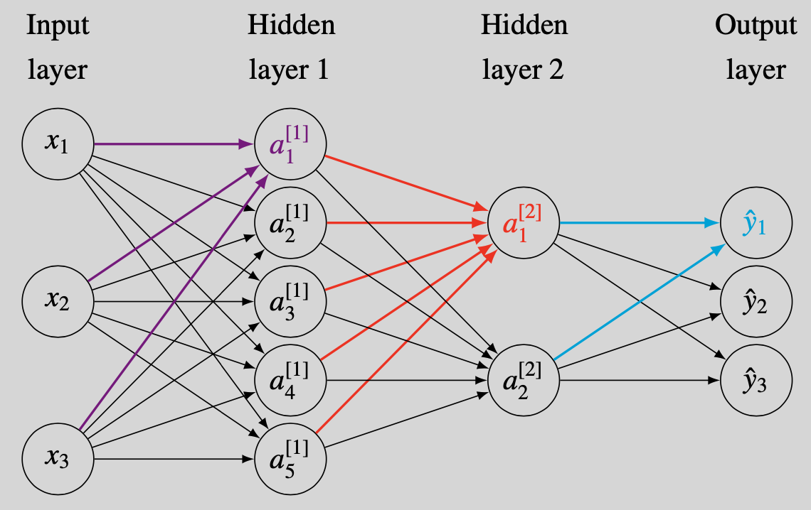
1. The value of neuron $a_1^{[1]}$ has similarities to a logistic regression. The three incoming arrows from $x_1$, $x_2$ and $x_3$ tell us to linearly combine these three inputs and to add the bias term $b_1^{[1]}$.¹ Stacking $\mathbf{x}=(x_1,x_2,x_3)^\prime$ and defining the weight vector $\mathbf{w}_{1}^{[1]}=(w_{11}^{[1]}, w_{12}^{[1]},w_{13}^{[1]})^\prime$, the linear combination is expressed compactly as $z_1^{[1]}=\mathbf{w}_{1}^{[1]\prime}\mathbf{x}+b_1^{[1]}$. Applying the sigmoid function $\Lambda(x)=\frac{1}{1+\exp(-x)}$, the result is $a_1^{[1]}=\Lambda(z_1^{[1]})$.

The other neurons in hidden layer 1 are computed in the same way. Each neuron will receive its own weight vector and bias. For $i=1,2,\ldots,5$, we have $z_i^{[1]}=\mathbf{w}_i^{[1]\prime}\mathbf{x}+ b_i^{[1]}$ and $a_i^{[1]}=\Lambda(z_i^{[1]})$.

2. Hidden layer 2 takes the values from the neurons in hidden layer 1 as inputs. For ease of notation, define $\mathbf{a}^{[1]}=(a_1^{[1]},a_2^{[1]},\ldots,a_5^{[1]})$. To compute $a_1^{[2]}$, calculate $z_1^{[2]}=\mathbf{w}_{1}^{[2]\prime}\mathbf{a}^{[1]}+b_1^{[2]}$ and $a_1^{[2]}=\Lambda(z_1^{[2]})$.

Similarly, $a_2^{[2]}=\Lambda(z_2^{[2]})$ with $z_2^{[2]}=\mathbf{w}_{2}^{[2]\prime}\mathbf{a}^{[1]}+b_2^{[2]}$.

3. The two-step computation for the output layer is somewhat different. As a start, we can still calculate the usual linear combinations $$ \begin{aligned} z_1^{[3]} &=\mathbf{w}_{1}^{[3]\prime}\mathbf{a}^{[2]}+b_1^{[3]}, \\ & \vdots \\ z_3^{[3]} &=\mathbf{w}_{3}^{[3]\prime}\mathbf{a}^{[2]}+b_3^{[3]},
   \end{aligned} $$ with $\mathbf{a}^{[2]}=(a_1^{[2]},a_2^{[2]})$. The subsequent transformation however should provide outcomes matching the type of data that is being modeled. For example, if $\hat{y}_1,\hat{y}_2,\hat{y}_3 \in \mathbb{R}$ (a multivariate regression), then no subsequent transformation is needed and we can simply use $\hat{y}_1=z_1^{[3]}$, $\hat{y}_2=z_2^{[3]}$ and $\hat{y}_3=z_3^{[3]}$. We pursue this case in the main text of this post. If the neural network output is used for classification, then a softmax output layer is more appropriate (Appendix C).

What are the benefits of neural networks?

The main advantage of a neural network is its flexible link between input features and output variable(s). That is, even highly nonlinear relationships in the data can be modelled throught these subsequent cascades of (1) linear combinations and (2) nonlinear transforms (through the sigmoid function).² This is particularly useful in data-rich environments when parametric relationship are just too restrictive.

Training a neural network

The values of the weight vectors and bias terms are still to be selected. We perform this selection using a cost function $\mathcal{C}$. This cost function quantifies the quality of a particular choice of weights and bias values. A higher cost indicates a worse choice of parameters. The evaluation of the cost function happens in the forward-propagation step. Backward-propagation suggests the direction in which the cost function is lower.

Forward-propagation

The forward propagation step evaluates the cost function $\mathcal{C}$. The procedure becomes more concise if we use matrix notation. For each layer $\ell=1,\ldots,L$, we stack the results for each neuron: $$ \mathbf{z}^{[\ell]} = \begin{bmatrix} z_1^{[\ell]} \\ \vdots \\ z_{n^{[\ell]}}^{[\ell]} \end{bmatrix} , \mathbf{b}^{[\ell]} = \begin{bmatrix} b_1^{[\ell]} \\ \vdots \\ b_{n^{[\ell]}}^{[\ell]} \end{bmatrix} , \mathbf{a}^{[\ell]} = \begin{bmatrix} a_1^{[\ell]} \\ \vdots \\ a_{n^{[\ell]}}^{[\ell]} \end{bmatrix} ,\text{and } \mathbf{W}^{[\ell]} = \begin{bmatrix} \mathbf{w}_1^{[\ell]\prime} \\ \vdots \\ \mathbf{w}_{n^{[\ell]}}^{[\ell]\prime}, \end{bmatrix} $$ where $n^{[\ell]}$ denotes the number of neurons in layer $\ell$. If we agree to apply the function $\Lambda$ elements-wise to vectors, then all computations of the previous section can be summarized by $$ \begin{aligned} \mathbf{z}^{[1]} &= \mathbf{W}^{[1]} \mathbf{x} + \mathbf{b}^{[1]}, &\mathbf{a}^{[1]} = \Lambda(\mathbf{z}^{[1]}), \\ \mathbf{z}^{[2]} &= \mathbf{W}^{[2]} \mathbf{a}^{[1]} + \mathbf{b}^{[2]}, &\mathbf{a}^{[2]} = \Lambda(\mathbf{z}^{[2]}), \\ \hat{\mathbf{y}} = \mathbf{z}^{[3]} &= \mathbf{W}^{[3]} \mathbf{a}^{[2]} + \mathbf{b}^{[3]}. \end{aligned} \label{eq:NNlayout} \tag{1} $$ It remains to compare the neural network output to the actual data. We let $\mathbf{y}=(y_1,y_2,y_3)^\prime$ denote the vector of observed outcomes. A possible cost function for this single-observation setting is the squared error $\| \hat{\mathbf{y}} - \mathbf{y} \|^2$.

In practice, we have multiple observations to determine $\mathbf{W}^{[1]}$, $\mathbf{W}^{[2]}$, $\mathbf{W}^{[3]}$, $\mathbf{b}^{[1]}$, $\mathbf{b}^{[2]}$, and $\mathbf{b}^{[3]}$. We assume a sample size of $T$ observations and enumerate the input-output pairs as $(\mathbf{x}^{(1)},\mathbf{y}^{(1)}),\ldots,(\mathbf{x}^{(T)},\mathbf{y}^{(T)})$. For each $t\in\{1,\ldots,T\}$, we now propagate the input $\mathbf{x}^{(t)}$ through the recursions in \eqref{eq:NNlayout} and find the implied prediction $\hat{\mathbf{y}}^{(t)}$. The cost function that takes all the samples into account is the Mean Square Error (MSE) defined as $$ MSE = \frac{1}{T} \sum_{t=1}^T \|\hat{\mathbf{y}}^{(t)} -\mathbf{y}^{(t)} \|^2. $$

---

NOTE: Instead of iterating through \eqref{eq:NNlayout} for each $\mathbf{x}^{(t)}$, a more efficient algorithm vectorizes this process. For example, after stacking $\mathbf{X}=[\mathbf{x}^{(1)} \cdots \mathbf{x}^{(T)}] \in \mathbb{R}^{3\times T}$, the matrix product $\mathbf{W}^{[1]}\mathbf{X}$ will immediately hold $\mathbf{W}^{[1]}\mathbf{x}^{(t)}$ in its $t$^th column.

---

Backward-propagation

The learning in the neural network is nothing but a series of successively better updates for $\mathbf{W}^{[1]}$, $\mathbf{W}^{[2]}$, $\mathbf{W}^{[3]}$, $\mathbf{b}^{[1]}$, $\mathbf{b}^{[2]}$, and $\mathbf{b}^{[3]}$. A popular method to perform these updates is gradient descent. Using a subscript ``$\{k\}$’’ to denote the $k$^th parameter update, we perform:

• Initialize $\mathbf{W}_{\{0\}}^{[1]}$, $\mathbf{W}_{\{0\}}^{[2]}$, $\mathbf{W}_{\{0\}}^{[3]}$, $\mathbf{b}_{\{0\}}^{[1]}$, $\mathbf{b}_{\{0\}}^{[2]}$, and $\mathbf{b}_{\{0\}}^{[3]}$ (more details later).
• For $\ell=1,\ldots,3$, update the parameters according to \begin{equation} \begin{aligned} \mathbf{W}_{\{k+1\}}^{[\ell]} &= \mathbf{W}_{\{k\}}^{[\ell]} - \alpha \frac{\partial \mathcal{C}}{\partial \mathbf{W}^{[\ell]}} \\ \mathbf{b}_{\{k+1\}}^{[\ell]} &= \mathbf{b}_{\{k\}}^{[\ell]} - \alpha \frac{\partial \mathcal{C}}{\partial \mathbf{b}^{[\ell]}} \end{aligned} \label{eq:GradientDescent} \tag{2} \end{equation} where
  • The learning rate $\alpha$ is a hyperparameter to be set by the researcher.
  • The terms $\frac{\partial \mathcal{C}}{\partial \mathbf{W}^{[\ell]}}$ and $\frac{\partial \mathcal{C}}{\partial \mathbf{b}^{[\ell]}}$ are the gradients of the cost function with respect to the weight matrices and bias vectors, respectively (see Appendix A for explanations on matrix and vector derivatives). The gradients in \eqref{eq:GradientDescent} are evaluated at the parameter values of iteration $k$.
• Stop updating upon convergence. Quantitative convergence criteria are difficult to formulate because we are generally not trying to find the global minimum of the cost function. The neural network is typically heavily parametrised and the global minimum is thus likely to overfit the data.³ We want to continue decreasing the training cost function as long as this also leads to decreases in the validation cost function.

The crucial components in \eqref{eq:GradientDescent} are $\frac{\partial \mathcal{C}}{\partial \mathbf{W}^{[\ell]}}$ and $\frac{\partial \mathcal{C}}{\partial \mathbf{b}^{[\ell]}}$ ($\ell=1,2,3$). These gradients are computed during backward-propagation. We will work our way backwards and start with the derivatives with respect to $\mathbf{W}^{[3]}$ and $\mathbf{b}^{[3]}$. For brevity, a single feature vector $\mathbf{x}$ is propagated as in \eqref{eq:NNlayout} to produce a single output vector $\hat{\mathbf{y}}$. The cost function is the squared error.

1. The cost function $\mathcal{C}=\| \mathbf{z}^{[3]} - \mathbf{y} \|^2$ depends on $\mathbf{W}^{[3]}$ and $\mathbf{b}^{[3]}$ through $\mathbf{z}^{[3]} = \mathbf{W}^{[3]} \mathbf{a}^{[2]} + \mathbf{b}^{[3]}$. We will have to use the chain rule. First, write $\mathcal{C}= \sum_{i=1}^{[n^L]} (z_{i}^{[3]}-y_i)^2$, calculate \begin{equation} \frac{\partial \mathcal{C}}{\partial z_i^{[3]}} = 2(z_i^{[3]}-y_i) = \left[ 2 (\mathbf{z}^{[3]} - \mathbf{y}) \right]_i \end{equation} and conclude that $\frac{\partial \mathcal{C}}{\partial \mathbf{z}^{[3]}}= 2 (\mathbf{z}^{[3]} - \mathbf{y})$. The gradient with respect to $\mathbf{b}^{[3]}$ is also $2 (\mathbf{z}^{[3]} - \mathbf{y})$ because $$ \begin{aligned} \frac{\partial \mathcal{C}}{\partial b_i^{[3]}} &= \sum_{j=1}^{[n^L]} \frac{\partial \mathcal{C}}{\partial z_j^{[3]}} \frac{\partial z_j^{[3]}}{\partial b_i^{[3]}} = \sum_{j=1}^{[n^L]} \frac{\partial \mathcal{C}}{\partial z_j^{[3]}} \frac{\partial}{\partial b_i^{[3]}} \left(\mathbf{w}_{j}^{[3]\prime} \mathbf{a}^{[2]}+b_j^{[3]}\right) \\ &= \sum_{j=1}^{[n^L]} \frac{\partial \mathcal{C}}{\partial z_j^{[3]}} \delta_{ij} = \frac{\partial \mathcal{C}}{\partial z_i^{[3]}} = \left[ 2 (\mathbf{z}^{[3]} - \mathbf{y}) \right]_i \end{aligned} $$ where we used the Kronecker delta \begin{equation} \delta_{ij} = \begin{cases} 1 & \quad \text{if } i=j,\\ 0 & \quad{ otherwise.} \end{cases} \end{equation} The calculation of $\frac{\partial \mathcal{C}}{\partial \mathbf{W}^{[3]}}$ is somewhat similar. Relabeling the summation index to avoid confusion with the subscripts of $w_{ij}$, we find $$ \begin{aligned} \frac{\partial \mathcal{C}}{\partial w_{ij}^{[3]}} &= \sum_{m=1}^{[n^L]} \frac{\partial \mathcal{C}}{\partial z_m^{[3]}} \frac{\partial z_m^{[3]}}{\partial b_i^{[3]}} = \sum_{m=1}^{[n^L]} \frac{\partial \mathcal{C}}{\partial z_m^{[3]}} \frac{\partial}{\partial w_{ij}^{[3]}} \left(\mathbf{w}_{m}^{[3]\prime} \mathbf{a}^{[2]}+b_m^{[3]}\right) \\ &= \sum_{m=1}^{[n^L]} \frac{\partial \mathcal{C}}{\partial z_m^{[3]}} \delta_{im} a_j^{[2]} = \frac{\partial \mathcal{C}}{\partial z_i^{[3]}} a_j^{[2]} = \left[ \frac{\partial \mathcal{C}}{\partial \mathbf{z}^{[3]}} \mathbf{a}^{[2]\prime} \right]_{ij}. \end{aligned} $$

For the parameters in layer 3, we find the following gradients: $$ \begin{aligned} \frac{\partial \mathcal{C}}{\partial \mathbf{b}^{[3]}} = \frac{\partial \mathcal{C}}{\partial \mathbf{z}^{[3]}} &= 2 (\mathbf{z}^{[3]} - \mathbf{y}), \\ \frac{\partial \mathcal{C}}{\partial \mathbf{W}^{[3]}} &= \frac{\partial \mathcal{C}}{\partial \mathbf{z}^{[3]}} \mathbf{a}^{[2]\prime}. \end{aligned} $$

2. Moving back one more layer, we are in layer 2. Four equations now determine the gradients with respect to $\mathbf{W}^{[2]}$ and $\mathbf{b}^{[2]}$, namely: $$ \begin{aligned} \mathcal{C} &=\| \mathbf{z}^{[3]} - \mathbf{y} \|^2, \\ \mathbf{z}^{[3]} &= \mathbf{W}^{[3]} \mathbf{a}^{[2]} + \mathbf{b}^{[3]}, \\ \mathbf{a}^{[2]} &= \Lambda(\mathbf{z}^{[2]})\\ \mathbf{z}^{[2]} &= \mathbf{W}^{[2]} \mathbf{a}^{[1]} + \mathbf{b}^{[2]}. \end{aligned} $$ Because we derived $\frac{\partial \mathcal{C}}{\partial \mathbf{z}^{[3]}}$ before, we can continue with $\frac{\partial \mathcal{C}}{\partial \mathbf{a}^{[2]}}$. Defining $w_{ij}^{[3]}$ as the $(i,j)$^th element of $\mathbf{W}^{[3]}$, the chain rule implies $$ \begin{aligned} \frac{\partial \mathcal{C}}{\partial a_i^{[2]}} &= \sum_{j=1}^{[n^L]} \frac{\partial \mathcal{C}}{\partial z_j^{[3]}} \frac{\partial z_j^{[3]}}{\partial a_i^{[2]}} = \sum_{j=1}^{[n^L]} \frac{\partial \mathcal{C}}{\partial z_j^{[3]}} \frac{\partial}{\partial a_i^{[2]}} \left(\mathbf{w}_{j}^{[3]\prime} \mathbf{a}^{[2]}+b_j^{[3]}\right) \\ &= \sum_{j=1}^{[n^L]} \frac{\partial \mathcal{C}}{\partial z_j^{[3]}} w_{ji}^{[3]} = \left[ \mathbf{W}^{[3]\prime} \frac{\partial \mathcal{C}}{\partial \mathbf{z}^{[3]}}\right]_i. \end{aligned} $$ We subsequently need to take care of $\mathbf{a}^{[2]}= \Lambda(\mathbf{z}^{[2]})$. This transformation is elements-wise implying that $a_i^{[2]}=\Lambda(z_{i}^{[2]})$ for $i\in\{1,2\}$ and thus $$ \begin{aligned} \frac{\partial \mathcal{C}}{\partial z_i^{[2]}} &= \frac{\partial \mathcal{C}}{\partial a_i^{[2]}} \frac{\partial a_i^{[2]}}{\partial z_i^{[2]}} = \frac{\partial \mathcal{C}}{\partial a_i^{[2]}} \Lambda’(z_i^{[2]}) \\ &= \frac{\partial \mathcal{C}}{\partial a_i^{[2]}} \Lambda(z_i^{[2]})\big(1-\Lambda(z_i^{[2]}) \big), \end{aligned} \label{eq:NonlinearTransformGradient} \tag{3} $$ where we used $\Lambda’(x)=\Lambda(x)\big(1-\Lambda(x)\big)$ (see this post on logistic regression). In matrix notation, we can use the Hadamard product (i.e. the elements-wise multiplication symbol “$\odot$”) to express \eqref{eq:NonlinearTransformGradient} as $\frac{\partial \mathcal{C}}{\partial \mathbf{z}^{[2]}} = \frac{\partial \mathcal{C}}{\partial \mathbf{a}^{[2]}} \odot \Lambda(\mathbf{z}^{[2]})\odot \big(\mathbf{1}-\Lambda(\mathbf{z}^{[2]})\big)$. Having computed the gradient with respect to $\mathbf{z}^{[2]}$, the calculations for $\frac{\partial \mathcal{C}}{\partial \mathbf{b}^{[2]}}$ and $\frac{\partial \mathcal{C}}{\partial \mathbf{W}^{[2]}}$ are exactly as in layer 3 because only another linear transformation $\mathbf{z}^{[2]} = \mathbf{W}^{[2]} \mathbf{a}^{[1]} + \mathbf{b}^{[2]}$ remains.

For the parameters in layer 2, we find the following gradients: $$ \begin{aligned} \frac{\partial \mathcal{C}}{\partial \mathbf{a}^{[2]}} &= \mathbf{W}^{[3]\prime} \frac{\partial \mathcal{C}}{\partial \mathbf{z}^{[3]}}, \\ \frac{\partial \mathcal{C}}{\partial \mathbf{b}^{[2]}}=\frac{\partial \mathcal{C}}{\partial \mathbf{z}^{[2]}} &= \frac{\partial \mathcal{C}}{\partial \mathbf{a}^{[2]}} \odot \Lambda(\mathbf{z}^{[2]})\odot \big(\mathbf{1}-\Lambda(\mathbf{z}^{[2]})\big), \\ \frac{\partial \mathcal{C}}{\partial \mathbf{W}^{[2]}} &= \frac{\partial \mathcal{C}}{\partial \mathbf{z}^{[2]}} \mathbf{a}^{[1]\prime}. \end{aligned} $$

3. Layer 1 is a fully-connected layer just like layer 2. Because the mathematical structure is identical to layer 2, the gradients follow immediately. We should only realized that the input variables to the first layer are $\mathbf{a}^{[0]}=\mathbf{x}$.

For the parameters in layer 1, we find the following gradients: $$ \begin{aligned} \frac{\partial \mathcal{C}}{\partial \mathbf{a}^{[1]}} &= \mathbf{W}^{[2]\prime} \frac{\partial \mathcal{C}}{\partial \mathbf{z}^{[2]}}, \\ \frac{\partial \mathcal{C}}{\partial \mathbf{b}^{[1]}}=\frac{\partial \mathcal{C}}{\partial \mathbf{z}^{[1]}} &= \frac{\partial \mathcal{C}}{\partial \mathbf{a}^{[1]}} \odot \Lambda(\mathbf{z}^{[1]})\odot \big(\mathbf{1}-\Lambda(\mathbf{z}^{[1]})\big), \\ \frac{\partial \mathcal{C}}{\partial \mathbf{W}^{[1]}} &= \frac{\partial \mathcal{C}}{\partial \mathbf{z}^{[1]}} \mathbf{a}^{[0]\prime}= \frac{\partial \mathcal{C}}{\partial \mathbf{z}^{[1]}} \mathbf{x}^{\prime}. \end{aligned} $$

---

NOTE: Our single-observation derivations generalize easily to a multiple-observation setting due to linearity of derivatives. Consider the input-output pairs $(\mathbf{x}^{(1)},\mathbf{y}^{(1)}),\ldots,(\mathbf{x}^{(T)},\mathbf{y}^{(T)})$ and $MSE = \frac{1}{T} \sum_{t=1}^T \|\hat{\mathbf{y}}^{(t)} -\mathbf{y}^{(t)} \|^2$. The gradient of the MSE with respect to say $\mathbf{W}^{[1]}$ is $$ \frac{\partial}{\partial \mathbf{W}^{[1]}} MSE = \frac{1}{T}\sum_{T=1}^T\frac{\partial}{\partial \mathbf{W}^{[1]}}\|\hat{\mathbf{y}}^{(t)} -\mathbf{y}^{(t)} \|^2. $$ The overall gradient is clearly just the average of all single-observation gradients. Theoretically, we can thus run the back-propagation algorithm for each observation and average. A practical implementation vectorizes this process to leverage the performance benefits of linear algebra libraries.

---

Remarks

• It is standard to initialize the gradient descent algorithm with $\mathbf{b}^{[1]}=\mathbf{b}^{[2]}=\mathbf{b}^{[3]}=\mathbf{0}$. This zero initialization should not be used for the weight matrix. Such a choice would imply $\frac{\partial \mathcal{C}}{\partial \mathbf{a}^{[2]}}=\frac{\partial \mathcal{C}}{\partial \mathbf{a}^{[1]}}=\mathbf{0}$ and all gradients would be zero. Gradient descent would not update any parameter. It is instead common practice to initialize the weight matrices with (small) random numbers. Concrete examples are the heuristic and normalized initializations in (1) and (16) of Glorot and Bengio (2010).
• The learning rate $\alpha$ is specified by the user. Common values are 0.1, 0.01, and 0.001. Determining a good choice for $\alpha$ typically requires some trial-and-error. If the learning rate is too high, then the cost function can oscillate strongly and even fail to converge. If the learning rate is too low, then cost function improvements are small and many iterations are needed.
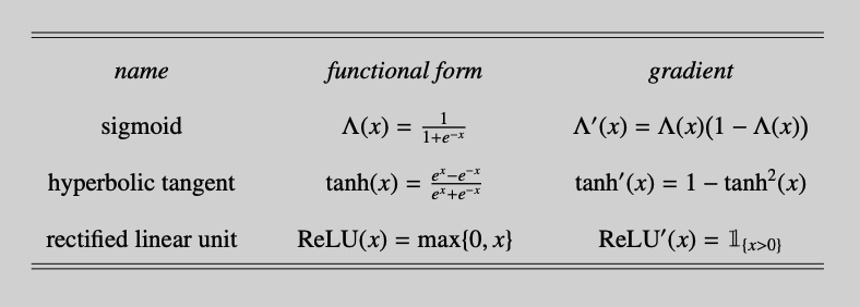
• The nonlinear functional transform in our neural network was the sigmoid function $\Lambda(x)=\frac{1}{1+\exp(-x)}$. Other activation functions can be used (Table 1). An inspection of the derivations shows that a change in activation function only impacts the backward propagation algorithm through \eqref{eq:NonlinearTransformGradient}. That is, if the new relationship is $\mathbf{a}^{[2]}=g(\mathbf{z}^{[2]})$, then \eqref{eq:NonlinearTransformGradient} becomes $\frac{\partial \mathcal{C}}{\partial z_i^{[2]}} = \frac{\partial \mathcal{C}}{\partial a_i^{[2]}} \frac{\partial a_i^{[2]}}{\partial z_i^{[2]}} = \frac{\partial \mathcal{C}}{\partial a_i^{[2]}} g’(z_i^{[2]})$.

• Several extensions of the baseline gradient descent algorithm have been proposed. Two of the most popular examples are:
  • The gradient descent updates can be smoothed across iterations. This can dampen oscilations and thus allow for higher learning rates (read: faster convergence). An example is the Adam optimizer by Kingma and Ba (2015) which keeps track of an exponential moving average of the gradient and squared gradient to smoothen the parameter update.
  • Mini batch gradient descent is particularly popular on larger datasets. With gradients being averages of the single-observation gradients, the gradient based on say 1,000 observations will already give a good indication of the direction of steepest descent. It is thus natural to update the parameters after evaluating the gradient based on a subset of the data (a mini batch). This effectively increases the parameter update speed.

Small illustration

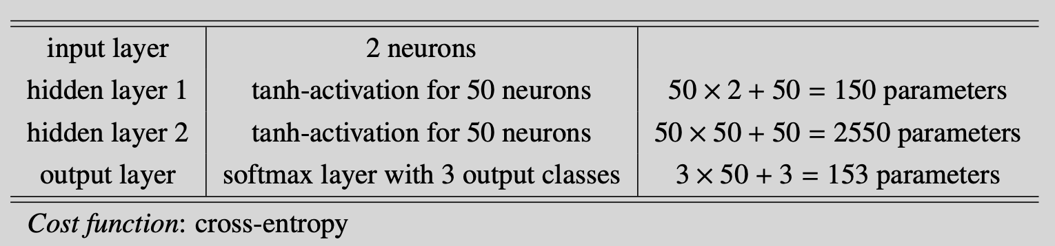
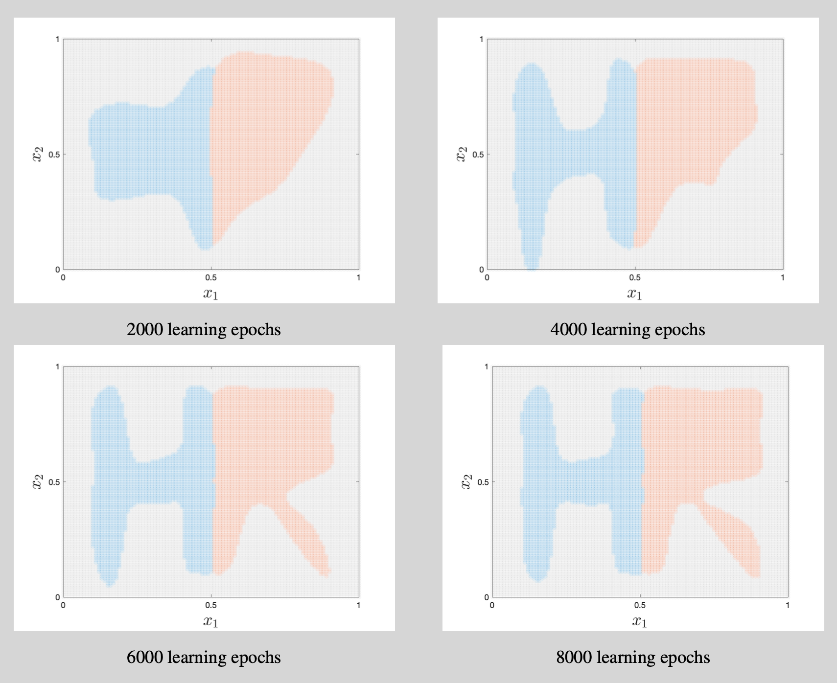
We use a neural network to classify the artificial data shown in Figure 2. The input feature vector $\mathbf{x}$ is 2-dimensional and there are three categories (the letter H, the letter R, and the background). This simulation design clearly generates a highly nonlinear mapping from input features to labels and a flexible classifier is thus needed. This justifies the use of a neural network. The details of the neural network implementation are listed in Table 2.

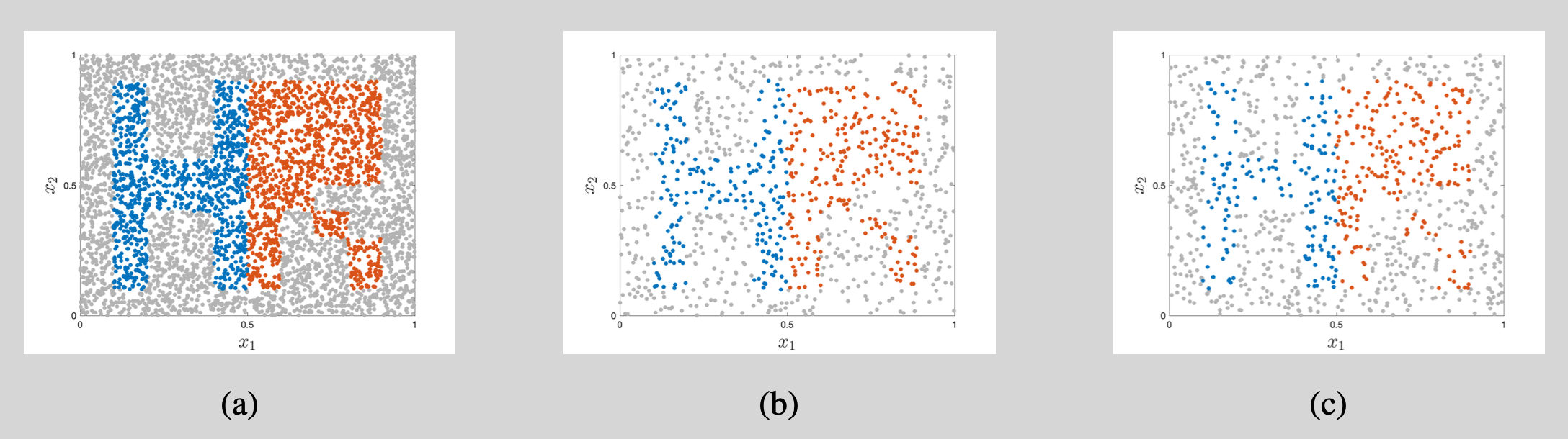
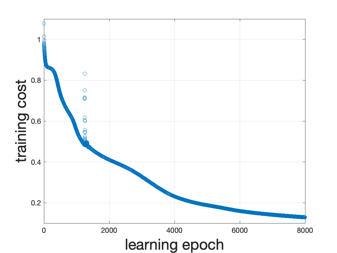
We initialize the weight matrices according to the ``normalized initialization’’ in Glorot and Bengio (2010) and start all bias vectors as $\boldsymbol{0}$. We subsequently use gradient descent with a learning rate of 0.2 to update the 2,853 parameters. In combination with the hyperbolic tangent activation functions, this results in a steady decrease of the cost function (Figure 3). The decrease is nearly monotonic except for a temporary spike in the cost function around learning epoch 1,260. Further debugging shows that this coincides with a sudden large increases of points in the left of the figure being classified as belonging to the blue category. This overshoot is corrected in subsequent iterations.

The learning process is further illustrated in Figure 4. The first 2,000 learning epochs provide a rather blurry outline of the letters H and R but subsequent parameter updates add more and more detail. As there are only tiny improvements during learning epochs 6,000 to 8,000 (both in the decision regions and in the cost function of Figure 3), we stop the learning process after 8,000 epochs.⁴

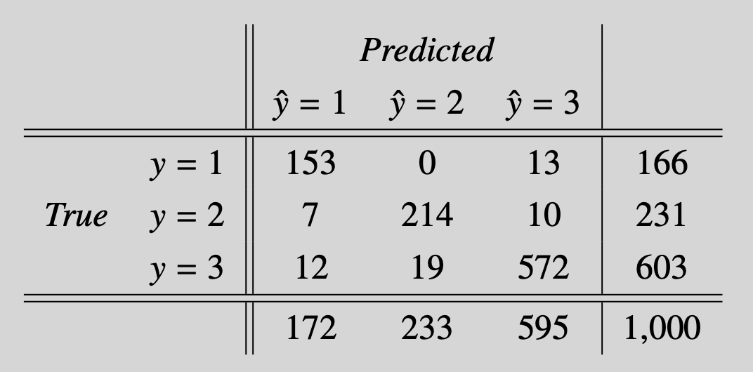
Finally, we verify the performance on the test data set. The overall performance is satisfactory with an accuracy of 93.9%. The confusion matrix (Table 3) shows that there is little mislabeling between the classes that define the H and R. Most errors are made when distinguishing the letters from the background.

Appendix A: Vector and matrix derivatives

As an $m$-dimensional vector can be interpreted as an $m\times 1$ matrix, it suffices to center this discussion around matrix derivatives. Defining the $m\times n$ matrix $\mathbf{A}$, \begin{equation} \mathbf{A} =\begin{bmatrix} a_{11} & \cdots & a_{1n} \\ \vdots & \ddots & \vdots \\ a_{m1} & \cdots & a_{mn} \end{bmatrix} \end{equation} and the function $f:\mathbb{R}^{m\times n}\to\mathbb{R}$, the matrix derivative $\frac{\partial f}{\partial \mathbf{A}}\in \mathbb{R}^{m\times n}$ is defined as \begin{equation} \frac{\partial f}{\partial \mathbf{A}} =\begin{bmatrix} \frac{\partial f}{\partial a_{11}} & \cdots & \frac{\partial f}{\partial a_{1n}} \\ \vdots & \ddots & \vdots \\ \frac{\partial f}{\partial a_{m1}} & \cdots & \frac{\partial f}{\partial a_{mn}} \end{bmatrix}. \end{equation} Two consequences of this definition should be stressed: (1) the dimensions of $\mathbf{A}$ and $\frac{\partial f}{\partial \mathbf{A}}$ are identical, and (2) the $(i,j)$^th element of $\frac{\partial f}{\partial \mathbf{A}}$ is $\frac{\partial f}{\partial a_{ij}}$. The second property is particularly interesting as it connects the calculation of a matrix derivative to the calculation of an ordinary partial derivative. The general recipe to compute matrix derivatives is therefore as follows:

1. Compute $\frac{\partial f}{\partial a_{ij}}$ for arbitrary $i$ and $j$.
2. The matrix derivative $\frac{\partial f}{\partial \mathbf{A}}$ is the matrix having $\frac{\partial f}{\partial a_{ij}}$ as its $(i,j)$^th element.

For example, let $f(\mathbf{A})=\mathbf{x}^\prime \mathbf{A}\mathbf{x}$ for $\mathbf{A}\in\mathbb{R}^{n\times n}$ and some fixed vector $\mathbf{x}\in\mathbb{R}^n$. As $\mathbf{x}^\prime \mathbf{A}\mathbf{x}= \sum_{k=1}^n \sum_{l=1}^n a_{kl} x_k x_l$, we have $\frac{\partial f}{\partial a_{ij}}= x_i x_j$. We conclude that $\frac{\partial}{\partial \mathbf{A}} \mathbf{x}^\prime \mathbf{A}\mathbf{x} = \mathbf{x} \mathbf{x}^\prime$, because \begin{equation} \left[\frac{\partial f}{\partial \mathbf{A}} \right]_{ij}= \frac{\partial f}{\partial a_{ij}} = x_i x_j = \left[\mathbf{x} \mathbf{x}^\prime \right]_{ij}. \end{equation}

Appendix B: Cross-entropy loss function

Consider a random sample $Y_1, Y_2,\ldots,Y_n$ of categorical data.⁵ For ease of notation, we will label these categories as $1,2,\ldots,K$ and denote the corresponding probabilities as $p_1,p_2,\ldots,p_K$. The associated likelihood is: $$ L(p_1,p_2,\ldots,p_K) = \prod_{i=1}^n p_1^{\mathbb{1}_{ \{ y_i=1 \} }} p_2^{\mathbb{1}_{ \{ y_i=2 \} }}\times \cdots \times p_K^{\mathbb{1}_{ \{ y_i=K \} }} $$ with $\mathbb{1}_{ \{ \mathcal{A} \} }$ denoting the indicator function for condition $\mathcal{A}$.⁶ The maximization of the likelihood is equal to the minimization of the cross-entropy loss function (the negative and logarithm of the previous likelihood) $$ -\sum_{i=1}^n \sum_{k=1}^K \mathbb{1}_{ \{ y_i = k \} } \log(p_k). $$ The intuition behind this formula is as follows. For any $y_i$, the indicator function inside the summation over $k$ will be equal to 1 exactly once (namely when $k$ equals the class label stored in $y_i$). The contribution of $- \sum_{k=1}^K \mathbb{1}_{ \{ y_i = k \} } \log(p_k)$ to the loss function is lowest if the probability for this class is as high as possible.

Appendix C: Classification output layer

We consider a neural network in which the output layer, layer $L$, should act as a classifier for $K$ classes. The combination of softmax activation and cross-entropy evaluation metric is very popular because (1) it works well in practice,⁷ and (2) it results in concise mathematical expressions for the back-propagation step.

The concrete implementation details are as follows. First, we match the number of neurons in the output layer to the number of output classes, i.e. $n^{[L]}=K$. The linear transformation towards the $L$^th layer is thus $\mathbf{z}^{[L]}= \mathbf{W}^{[L]} \mathbf{a}^{[L-1]} + \mathbf{b}^{[L]}$ with $\mathbf{W}^{[L]}\in\mathbb{R}^{K\times n^{[L-1]}}$ and $\mathbf{b}\in\mathbb{R}^{K}$. Second, we convert $\mathbf{z}^{[L]}$ into a $K$-dimensional vector of probabilities using the softmax activation. That is, we calculate \begin{equation} p_i^{[L]} = \frac{ \exp(z_i^{[L]}) }{ \sum_{k=1}^{K} \exp(z_k^{[L]}) }, \qquad\text{for }i=1,2,\ldots,K, \label{eq:SoftmaxActivation} \tag{2} \end{equation} and stack $\mathbf{p}^{[L]} = (p_1^{[L]},\ldots,p_K^{[L]})^\prime$. The crucial component of \eqref{eq:SoftmaxActivation} is the use of the exponential function to obtain positive outcomes and the standardization in the denominator to ensure that probabilities add to $1$.

Finally, let us look at the back-propagation step. For brevity of notation, we will consider a single outcome observation $y$ and omit superscripts referring to the final layer. The cost function and softmax activation are thus $C=-\sum_{k=1}^K \mathbb{1}_{ \{ y = k \} } \log(p_k)$ and $p_i = \exp(z_i) / \sum_{\kappa=1}^{K} \exp(z_\kappa)$ $(i=1,2,\ldots,K)$, respectively. We are interested in $\frac{\partial C}{\partial \mathbf{z}}$.

Motivated by Appendix A, we derive the $j$^th component of $\frac{\partial C}{\partial \mathbf{z}}$. We have $$ \begin{aligned} \frac{\partial C}{\partial z_j} &=-\sum_{k=1}^K \mathbb{1}_{ \{ y = k \} } \frac{1}{p_k} \frac{ \partial p_k}{\partial z_j} \\ &=-\sum_{k=1}^K \mathbb{1}_{ \{ y = k \} } \frac{1}{p_k} \left(\frac{ \exp(z_j) }{ \sum_{\kappa=1}^{K} \exp(z_\kappa) }\mathbb{1}_{ \{ j=k \}} - \frac{ \exp(z_k) \exp(z_j) }{ ( \sum_{\kappa=1}^{K} \exp(z_\kappa) )^2 } \right) \\ &=-\sum_{k=1}^K \mathbb{1}_{ \{ y = k \} } \left(\mathbb{1}_{ \{ j=k \}} - p_j \right) = p_j- \mathbb{1}_{ \{ y=j \}} . \end{aligned} $$ In conclusion, if we use one-hot encoding for the outcome $y$, then $\frac{\partial C}{\partial \mathbf{z}} = \mathbf{p}-\mathbf{y}$. Having calculated the derivative with respect to $\mathbf{z}$, the resulting derivates for $\mathbf{W}$ and $\mathbf{b}$ take the usual form.

References

X. Glorot and Y. Bengio (2010), Understanding the Difficulty of Training Deep Feedforward Neural Networks, Proceedings of the 13^th International Conference on Artificial Intelligence and Statistics (AISTATS)

N.J. Guliyevand V.E. Ismailov (2018), On the Approximation by Single Hidden Layer Feedforward Neural Networks with Fixed Weights, Neural Networks

D.P. Kingma and J. Ba (2015), Adam: A Method for Stochastic Optimization, arXiv:1412.6980

S.A. Solla, E. Levin and M. Fleisher (1988), Accelerated Learning in Layered Neural Networks, Complex Systems

Notes